

The first four parts presented LTN’s mechanisms on toy examples. This case study puts them to the test on a harder problem: recognizing handwritten digits without ever seeing the label of a single digit.
The model is given two images of digits, and a single piece of information: their sum. From there, it has to learn to recognize each digit. We then compare this LTN with a purely supervised baseline, which learns to predict the sum directly, with no logical knowledge at all.
Why this example?
This problem was not picked at random. It is a classic case in the neuro-symbolic literature, introduced by the DeepProbLog paper (Manhaeve et al., 2018) and taken up in the original LTN paper. Three qualities make it a good testbed for comparison:
- it isolates the difficulty we care about. Recognizing a handwritten digit is a task neural networks handle well. The challenge here is to combine several pieces of information to produce an answer, which lets us observe what logic brings;
- the rule is known: the answer is the sum of the digits. But the two approaches use it differently: the baseline has to learn it from the examples, whereas the LTN states it explicitly as a logical rule;
- the difficulty is easy to tune, by increasing the number of digits to combine. We can then see how both approaches behave as the problem gets harder.
The problem
We consider two tasks, built from the MNIST dataset of handwritten digits.
Adding two digits. Consider the predicate , where and are images of digits and an integer equal to their sum. It must estimate whether the addition is valid: is valid, is not. Here, simply means “an image of the digit ”, not a logical function.
Adding two-digit numbers. The predicate becomes:
where each list represents a two-digit number. The first addition below is valid, the second is not:
The neuro-symbolic approach is to learn a single-digit classifier, and to rely on what we already know about addition. If a predicate gives the likelihood that image represents digit , the addition is written in LTN as:
The difficulty is that no label of an individual digit is given during training: only the sum of each pair is known. The classifier is therefore never trained directly on its own task. Its output remains latent information, used only by the logic. This is not a problem for LTN, since the gradient flows through the whole logical structure, all the way to the classifier’s weights.
The LTN theory
Domains:
- : the MNIST digit images;
- : the integers that are results of additions;
- : the digits from 0 to 9.
Variables:
- range over images, over results and over digits;
- , , .
Predicate: , the single-digit classifier, which returns the probability that image represents digit . Its input domain is .
Axioms. For adding two digits:
and for adding two-digit numbers:
Two mechanisms from part 2 come back:
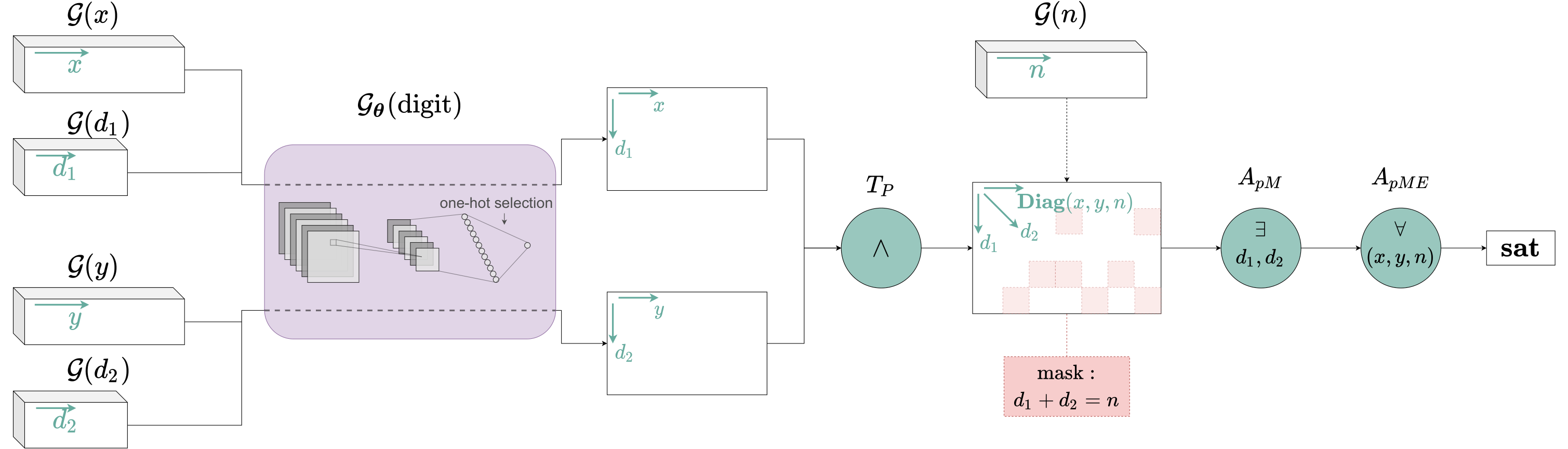
- diagonal quantification ensures that the -th elements of , and match: is a triple from the dataset. LTN aggregates each pair of images with its own result, not with any result;
- guarded quantification keeps, among the possible digits, only those whose sum can give the result. This is how the symbolic information enters the system.
Grounding:
- : MNIST images are 28 × 28 grayscale pixels, and their values, from 0 to 255 initially, are scaled to ;
- and ;
- and : the three variables have the same number of examples, since matches them one to one;
- ;
- , where is a convolutional network with 10 outputs, one per digit. Unlike in the previous parts, is a raw integer here, which converts at evaluation time.
The figure from the original paper sums up the full computation graph for adding two digits:
The dataset
MNIST contains 70,000 images: 60,000 for training and 10,000 for testing. We need to derive an addition dataset from it.
- For two digits, the first 30,000 training images serve as left operands, the next 30,000 as right operands, and the sum of their labels is the target. The same is done for the test set.
- For two two-digit numbers, the training set is split into four groups of 15,000 images: the first two form the digits of the first number, the last two those of the second.
import torch
import pandas as pd
import torchvision

def get_mnist_dataset_for_digits_addition(single_digit=True):
    """
    Prepares the dataset for the MNIST digit addition example (single digit or multiple digits)
    de l'article LTN.

    :param single_digit: whether the dataset has to be generated for the single digit case
        or the multi digit case (see the specification above to understand the difference between the two).
    :return: a pair of two elements. The first is the training set, the second the test set.
        Each one is a list containing:
        1. a list [left_operands, right_operands], where left_operands is a list of MNIST images
           used as the left operand of the addition, and right_operands as the right operand;
        2. a list containing the sum of the labels of the images of point 1. The label of the left operand
           is added to that of the right operand, forming the target of the addition task.
    This describes the result for the single digit case. In the multi digit case, the list of point 1
    has 4 elements, since four digits are involved in each addition (two to represent
    the first operand, two for the second).
    """
    if single_digit:
        n_train_examples = 30000
        n_test_examples = 5000
        n_operands = 2
    else:
        n_train_examples = 15000
        n_test_examples = 2500
        n_operands = 4

    mnist_train = torchvision.datasets.MNIST("./datasets/", train=True, download=True,
                                             transform=torchvision.transforms.ToTensor())
    mnist_test = torchvision.datasets.MNIST("./datasets/", train=False, download=True,
                                            transform=torchvision.transforms.ToTensor())

    train_imgs, train_labels, test_imgs, test_labels = mnist_train.data, mnist_train.targets, \
                                                       mnist_test.data, mnist_test.targets

    train_imgs, test_imgs = train_imgs / 255.0, test_imgs / 255.0

    train_imgs, test_imgs = torch.unsqueeze(train_imgs, 1), torch.unsqueeze(test_imgs, 1)

    imgs_operand_train = [train_imgs[i * n_train_examples:i * n_train_examples + n_train_examples]
                          for i in range(n_operands)]
    labels_operand_train = [train_labels[i * n_train_examples:i * n_train_examples + n_train_examples]
                            for i in range(n_operands)]

    imgs_operand_test = [test_imgs[i * n_test_examples:i * n_test_examples + n_test_examples]
                         for i in range(n_operands)]
    labels_operand_test = [test_labels[i * n_test_examples:i * n_test_examples + n_test_examples]
                           for i in range(n_operands)]

    if single_digit:
        label_addition_train = labels_operand_train[0] + labels_operand_train[1]
        label_addition_test = labels_operand_test[0] + labels_operand_test[1]
    else:
        label_addition_train = 10 * labels_operand_train[0] + labels_operand_train[1] + \
                               10 * labels_operand_train[2] + labels_operand_train[3]

        label_addition_test = 10 * labels_operand_test[0] + labels_operand_test[1] + \
                              10 * labels_operand_test[2] + labels_operand_test[3]

    train_set = [torch.stack(imgs_operand_train, dim=1), label_addition_train]
    test_set = [torch.stack(imgs_operand_test, dim=1), label_addition_test]

    return train_set, test_set

# dataset for the single digit case
single_d_train_set, single_d_test_set = get_mnist_dataset_for_digits_addition(single_digit=True)
# dataset for the multi digit case
multi_d_train_set, multi_d_test_set = get_mnist_dataset_for_digits_addition(single_digit=False)
Understanding the structure of the data
There are three levels to tell apart: an example, the dataset and a batch.
An example is one addition. For , it contains two images and one label:
Example
├── image of the digit 3
├── image of the digit 7
└── label = 10
Each MNIST image is a tensor of shape (1, 28, 28): one channel (grayscale), 28 pixels high, 28 wide. The two images of an example are grouped in a tensor of shape (2, 1, 28, 28).
The dataset gathers examples. The images form a single tensor of shape (m, 2, 1, 28, 28), and the labels a tensor of shape (m,), with a direct correspondence: images[i] and labels[i] describe the same addition.
(m, 2, 1, 28, 28)
 ↑  ↑
 │  └── number of images per example
 └───── number of examples
This is exactly what single_d_train_set holds: a list of two elements, the images at [0] and the labels at [1]. single_d_train_set[0][0] first selects the images, then the first example: a (2, 1, 28, 28) tensor. single_d_train_set[1][0] selects the label of that same example, a scalar.
A batch gathers examples: its images have shape (B, 2, 1, 28, 28) and its labels (B,). The first two dimensions must not be confused: (32, 2, 1, 28, 28) represents 32 additions, each described by 2 images.
For adding two-digit numbers, the principle is the same with 4 images per example: (m, 4, 1, 28, 28) for the dataset, (B, 4, 1, 28, 28) for a batch.
Let’s display the first training example for adding two digits:
import matplotlib.pyplot as plt
first_example_images = single_d_train_set[0][0]
first_example_label = single_d_train_set[1][0]

print("The operands are shown in the following images:")
fig = plt.figure()
ax = fig.add_subplot(1, 2, 1)
imgplot = plt.imshow(first_example_images[0].permute(1, 2, 0))
ax.set_title('First operand')
ax = fig.add_subplot(1, 2, 2)
imgplot = plt.imshow(first_example_images[1].permute(1, 2, 0))
ax.set_title('Second operand')
plt.show()
print("The target label (the sum) for these operands is: %d" % first_example_label.item())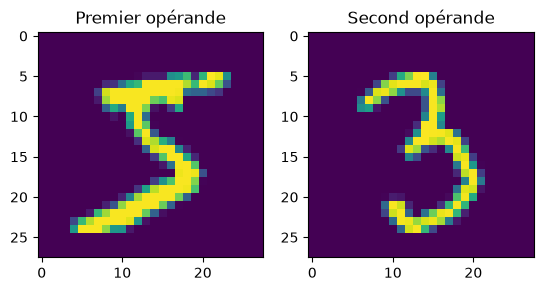
The operands are shown in the following images:
The target label (the sum) for these operands is: 8
A 5 and a 3, adding up to 8: this is the only information the model will get for this example. (The plot titles were generated by the notebook, which is in French.)
The LTN model
We need to define the predicate, the variables to , the connectives, the quantifiers and SatAgg. Connectives and quantifiers follow the product configuration seen in part 3.
The predicate relies on two models:
- the first is a CNN that returns the logits of the ten classes for an image ;
- the second takes a pair , computes the logits with the first, applies a softmax, and returns the probability of class : the likelihood that image represents digit .
We keep the two separate because we need both outputs: the logits are used to measure classification accuracy, and the probabilities are read as degrees of truth to compute the satisfaction of the knowledge base.
The variables to range over the ten digits, . Unlike the one-hot labels of the previous parts, these are raw integer indices: torch.gather directly selects the probability of index .
from torch.nn.init import xavier_uniform_, normal_, kaiming_uniform_
import ltn

# we define the variables
d_1 = ltn.Variable("d_1", torch.tensor(range(10)))
d_2 = ltn.Variable("d_2", torch.tensor(range(10)))
# only used in the multi digit case
d_3 = ltn.Variable("d_3", torch.tensor(range(10)))
d_4 = ltn.Variable("d_4", torch.tensor(range(10)))

# we define the digit predicate
class MNISTConv(torch.nn.Module):
    """
    CNN that returns embeddings for MNIST images.
    Arguments:
        conv_channels_sizes: tuple containing the number of channels of the convolutional layers of the model. The first
        element must be the number of input channels of the first layer, the last one the number of output
        channels of the last layer. The number of layers built is `len(conv_channels_sizes) - 1`;

        kernel_sizes: tuple containing the sizes of the kernels used in the convolutional layers;

        linear_layers_sizes: tuple containing the sizes of the final dense layers of the architecture. The first
        element must be the number of input features of the first dense layer, the last one the number of
        output features of the last one. The number of layers built is `len(linear_layers_sizes) - 1`.
    """
    def __init__(self, conv_channels_sizes=(1, 6, 16), kernel_sizes=(5, 5), linear_layers_sizes=(256, 100)):
        super(MNISTConv, self).__init__()
        self.conv_layers = torch.nn.ModuleList([torch.nn.Conv2d(conv_channels_sizes[i - 1], conv_channels_sizes[i],
                                                                kernel_sizes[i - 1])
                                                  for i in range(1, len(conv_channels_sizes))])
        self.elu = torch.nn.ELU()  # activation used everywhere, as in baselines.py (Keras, activation="elu")
        self.maxpool = torch.nn.MaxPool2d((2, 2))
        self.linear_layers = torch.nn.ModuleList([torch.nn.Linear(linear_layers_sizes[i - 1], linear_layers_sizes[i])
                                                  for i in range(1, len(linear_layers_sizes))])

        self.init_weights()

    def forward(self, x):
        for conv in self.conv_layers:
            x = self.elu(conv(x))
            x = self.maxpool(x)
        x = torch.flatten(x, start_dim=1)
        for linear in self.linear_layers:
            x = self.elu(linear(x))
        return x

    def init_weights(self):
        r"""Initializes the weights of the network.
        All weights (convolutional and dense) are initialized with :py:func:`torch.nn.init.xavier_uniform_`
        (equivalent to Keras's default "glorot_uniform" initializer, used in baselines.py),
        biases with :py:func:`torch.nn.init.zeros_`.
        """
        for layer in self.conv_layers:
            xavier_uniform_(layer.weight)
            torch.nn.init.zeros_(layer.bias)

        for layer in self.linear_layers:
            xavier_uniform_(layer.weight)
            torch.nn.init.zeros_(layer.bias)


class SingleDigitClassifier(torch.nn.Module):
    """
    Model that classifies an MNIST digit image among 10 possible classes. It returns the logits, an
    unnormalized output. Architecture faithful to baselines.SingleDigit: convolutional part (MNISTConv, ELU), then a
    hidden dense layer (ELU), then the final classification layer
    Arguments:
        layers_sizes: tuple containing the sizes of the final dense layers of the architecture. The first
        element must be the number of input features of the first layer, the last one the number of
        output features of the last one. The number of layers built is `len(layers_sizes) - 1`.
    """
    def __init__(self, layers_sizes=(100, 84, 10)):
        super(SingleDigitClassifier, self).__init__()
        self.mnistconv = MNISTConv()  # convolutional part of the architecture
        self.elu = torch.nn.ELU()  # activation of the hidden dense layers
        self.linear_layers = torch.nn.ModuleList([torch.nn.Linear(layers_sizes[i - 1], layers_sizes[i])
                                                  for i in range(1, len(layers_sizes))])
        self.init_weights()

    def forward(self, x):
        x = self.mnistconv(x)
        for i in range(len(self.linear_layers) - 1):
            x = self.elu(self.linear_layers[i](x))
        return self.linear_layers[-1](x)  # a sigmoid or a softmax must be applied on the last layer

    def init_weights(self):
        """Initializes the weights of the dense layers of the network.
        Weights are initialized with :py:func:`torch.nn.init.xavier_uniform_`,
        biases with :py:func:`torch.nn.init.zeros_`.
        """
        for layer in self.linear_layers:
            xavier_uniform_(layer.weight)
            torch.nn.init.zeros_(layer.bias)


class LogitsToPredicate(torch.nn.Module):
    """
    This model wraps a logits model, which computes the class logits for an input image x.
    The idea is to keep logits and probabilities separate: the logits model returns the logits for an example,
    while this model returns the probabilities computed from those logits.

    Concretely, it takes an image x and a class label d as input. It applies the logits model
    to x to get the logits, then a softmax function to get the probability of each class. Finally, it
    only returns the probability of class d, selected directly by indexing rather than
    by a product with a one-hot vector, since d is a raw integer index here.
    """
    def __init__(self, logits_model):
        super(LogitsToPredicate, self).__init__()
        self.logits_model = logits_model
        self.softmax = torch.nn.Softmax(dim=1)

    def forward(self, x, d):
        logits = self.logits_model(x)
        probs = self.softmax(logits)
        out = torch.gather(probs, 1, d)
        return out

# single digit
cnn_s_d = SingleDigitClassifier()
Digit_s_d = ltn.Predicate(LogitsToPredicate(cnn_s_d)).to(ltn.device)
# multiple digits
cnn_m_d = SingleDigitClassifier()
Digit_m_d = ltn.Predicate(LogitsToPredicate(cnn_m_d)).to(ltn.device)

# we define the connectives, quantifiers, and SatAgg
And = ltn.Connective(ltn.fuzzy_ops.AndProd())
Exists = ltn.Quantifier(ltn.fuzzy_ops.AggregPMean(p=2), quantifier="e")
Forall = ltn.Quantifier(ltn.fuzzy_ops.AggregPMeanError(p=2), quantifier="f")
SatAgg = ltn.fuzzy_ops.SatAgg()
The baseline
For comparison, we also train a standard network, with no logic. It encodes each image with the same convolutional trunk as the LTN (weights shared across operands), concatenates the representations, then predicts the sum directly. It is a 19-class classification for two digits (0 to 18), and a 199-class one for two two-digit numbers (0 to 198).
# ===============================================
# BASELINE (standard CNN, no logic)
# ===============================================

class BaselineNet(torch.nn.Module):
    """
    "Baseline" network: encodes each operand image with the SAME convolutional trunk
    (MNISTConv, shared weights, siamese architecture), concatenates the embeddings, then a
    hidden dense layer (ELU) and a final classification layer (raw logits) directly predict
    the class of the result (the sum), with no intermediate logical predicates.
    """
    def __init__(self, n_operands, n_classes, embedding_dim=100, hidden_dim=100):
        super(BaselineNet, self).__init__()
        self.encoder = MNISTConv()  # convolutional trunk shared by the operands
        self.fc1 = torch.nn.Linear(embedding_dim * n_operands, hidden_dim)
        self.fc2 = torch.nn.Linear(hidden_dim, n_classes)
        self.elu = torch.nn.ELU()
        self.init_weights()

    def init_weights(self):
        xavier_uniform_(self.fc1.weight)
        torch.nn.init.zeros_(self.fc1.bias)
        xavier_uniform_(self.fc2.weight)
        torch.nn.init.zeros_(self.fc2.bias)

    def forward(self, images_list):
        embeddings = [self.encoder(img) for img in images_list]
        x = torch.cat(embeddings, dim=1)
        x = self.elu(self.fc1(x))
        return self.fc2(x)  # raw logits


# baseline for the single digit case: sum of 2 digits -> 19 classes (0 to 18)
baseline_s_d = BaselineNet(n_operands=2, n_classes=19, hidden_dim=84).to(ltn.device)
# baseline for the multi digit case: sum of two 2-digit numbers -> 199 classes (0 to 198)
baseline_m_d = BaselineNet(n_operands=4, n_classes=199, hidden_dim=128).to(ltn.device)
Finally, we define a data loader, for training and testing on both tasks:
import numpy as np

# standard PyTorch data loader, for training and testing the model
class DataLoader(object):
    def __init__(self,
                 fold,
                 batch_size=1,
                 shuffle=True):
        self.fold = fold
        self.batch_size = batch_size
        self.shuffle = shuffle

    def __len__(self):
        return int(np.ceil(self.fold[0].shape[0] / self.batch_size))

    def __iter__(self):
        n = self.fold[0].shape[0]
        idxlist = list(range(n))
        if self.shuffle:
            np.random.shuffle(idxlist)

        for _, start_idx in enumerate(range(0, n, self.batch_size)):
            end_idx = min(start_idx + self.batch_size, n)
            digits = self.fold[0][idxlist[start_idx:end_idx]]
            addition_labels = self.fold[1][idxlist[start_idx:end_idx]]

            yield digits, addition_labels

# create the training and test loaders
single_train_loader = DataLoader(single_d_train_set, 32, shuffle=True)
single_test_loader = DataLoader(single_d_test_set, 32, shuffle=False)
multi_d_train_loader = DataLoader(multi_d_train_set, 32, shuffle=True)
multi_d_test_loader = DataLoader(multi_d_test_set, 32, shuffle=False)
The two approaches therefore share everything, except how they learn:
| LTN | Baseline | |
|---|---|---|
| Input data | identical | identical |
| Convolutional trunk | identical architecture | identical architecture |
| Batch size | 32 | 32 |
| Optimizer | Adam, | Adam, |
| Objective | maximize satisfaction | minimize the error on the sum |
| Loss function | cross-entropy | |
| Logical knowledge | none | |
| Epochs | 20 | 30 |
The baseline is trained longer (30 epochs versus 20), following the protocol of the paper.
Learning
Let be the set of examples. The objective is:
that is, each formula of is evaluated on the examples of with the model of parameters , then aggregates these satisfactions. In practice, the optimizer minimizes, on a mini-batch drawn from :
Since the knowledge base here contains a single axiom, SatAgg is not used explicitly: applied to a single value, it would return it unchanged. The result of Forall directly serves as the satisfaction level.
The schedule of . The parameter of the existential quantifier increases in steps during training: , then 2, then 4, then 6. At the start, the classifier is close to random. A high would focus the whole gradient on the best hypothesis of the moment, and could reinforce a wrong combination of digits just because it has the highest confidence at initialization. A low spreads the gradient over all plausible combinations and lets the right signal emerge; the focus is then tightened once the classifier becomes reliable. This is a direct application of the trade-off seen in part 3.
Accuracy is measured by predicting each digit with the CNN, then checking that the reconstructed addition gives the right result.
Here is the core of training, the formula evaluated on each batch:
sat_agg = Forall(
    ltn.diag(images_x, images_y, labels_z),
    Exists(
        [d_1, d_2],
        And(Digit_s_d(images_x, d_1), Digit_s_d(images_y, d_2)),
        cond_vars=[d_1, d_2, labels_z],
        cond_fn=lambda d1, d2, z: torch.eq(d1.value + d2.value, z.value),
        p=p
    )).value
It reads: for each example, there must be two digits that match the two images and whose sum equals the observed result.
How this formula learns the digits, step by step
Take a batch of two examples: and .
1. The data. The first images go into images_x, the second ones into images_y, the results into labels_z, each with a batch dimension of 2. ltn.diag(images_x, images_y, labels_z) keeps the triples aligned: (image of 2, image of 3, 5) and (image of 1, image of 4, 5), without crossing the images of one example with the result of another.
2. The Digit predicate. For an image, the CNN produces logits, then a softmax gives a distribution over the ten digits, for example:
d      0     1     2     3     4     5   ...
p_d   0.01  0.02  0.90  0.01  0.01  0.01 ...
Digit_s_d(x, d) is the probability of digit : here , a high degree of truth for “image represents a 2”.
3. The admissible pairs. and each range over , giving 100 possible pairs. The cond_fn mask only keeps those whose sum equals the result. For : . This mask recognizes nothing in the pixels: it only says which combinations of digits are compatible with the label.
4. The conjunction. For each admissible pair, And multiplies the two probabilities. Suppose the network gives 0.90 to the 2 for the first image and 0.85 to the 3 for the second:
AndProd | |||
|---|---|---|---|
| (0, 5) | 0.01 | 0.02 | 0.0002 |
| (1, 4) | 0.02 | 0.01 | 0.0002 |
| (2, 3) | 0.90 | 0.85 | 0.7650 |
| (3, 2) | 0.01 | 0.03 | 0.0003 |
| (4, 1) | 0.01 | 0.02 | 0.0002 |
| (5, 0) | 0.01 | 0.01 | 0.0001 |
Several pairs are mathematically correct, and the constraint alone is not enough to decide. The Digit predicate brings the visual information: the logic says , and the CNN says which values are the most plausible given the images.
5. The existential. Exists aggregates the six values with pMean: for , . The result is higher when at least one explanation is very plausible, here the pair (2, 3).
6. The universal. Exists produces one satisfaction per example, then Forall aggregates them with pMeanError into an overall satisfaction for the batch. A badly explained example weighs more than one that is already well satisfied.
7. The gradient. This whole chain is differentiable: CNN weights → logits → softmax → Digit → And → Exists → Forall. The gradient flows back the other way. For the pair (2, 3), the satisfaction is , with and , so and : the gradient acts on the probabilities, then on the logits, then on the CNN weights.
8. Why the digits end up being learned. A single example like is not enough to identify both digits. The information comes from all the examples together: a 2 also appears in , , … The hypothesis “this is a 2” stays consistent with all these additions, while a wrong hypothesis becomes incompatible with a growing number of examples. Since the same CNN is shared by every example, the gradients of all these constraints add up, and push it toward distributions where for images of 2. The individual digits act as latent variables: the CNN provides the predictions, the logic provides the constraints.
Adding two digits
We train the LTN for 20 epochs:
history_single = {"train_loss": [], "train_sat": [], "train_acc": [],
                   "test_loss": [], "test_sat": [], "test_acc": []}

optimizer = torch.optim.Adam(Digit_s_d.parameters(), lr=0.001)

for epoch in range(20):
    # schedule of the parameter p for the existential quantifier, as described in the LTN paper
    if epoch in range(0, 4):
        p = 1
    if epoch in range(4, 8):
        p = 2
    if epoch in range(8, 12):
        p = 4
    if epoch in range(12, 20):
        p = 6
    train_loss, test_loss = 0.0, 0.0
    train_sat, test_sat = 0.0, 0.0
    train_acc, test_acc = 0.0, 0.0
    # training step
    cnn_s_d.train()
    for batch_idx, (operand_images, addition_label) in enumerate(single_train_loader):
        optimizer.zero_grad()
        # ground the variables with the current batch data
        images_x = ltn.Variable("x", operand_images[:, 0])
        images_y = ltn.Variable("y", operand_images[:, 1])
        labels_z = ltn.Variable("z", addition_label)
        sat_agg = Forall(
            ltn.diag(images_x, images_y, labels_z),
            Exists(
                [d_1, d_2],
                And(Digit_s_d(images_x, d_1), Digit_s_d(images_y, d_2)),
                cond_vars=[d_1, d_2, labels_z],
                cond_fn=lambda d1, d2, z: torch.eq(d1.value + d2.value, z.value),
                p=p
            )).value
        loss = 1. - sat_agg
        loss.backward()
        optimizer.step()
        train_loss += loss.item()
        train_sat += sat_agg.item()
        # compute the training accuracy
        predictions_x = torch.argmax(cnn_s_d(operand_images[:, 0].to(ltn.device)), dim=1)
        predictions_y = torch.argmax(cnn_s_d(operand_images[:, 1].to(ltn.device)), dim=1)
        predictions = predictions_x + predictions_y
        train_acc += torch.count_nonzero(torch.eq(addition_label.to(ltn.device), predictions)) / predictions.shape[0]
    train_loss = train_loss / len(single_train_loader)
    train_sat = train_sat / len(single_train_loader)
    train_acc = train_acc / len(single_train_loader)

    # test step
    cnn_s_d.eval()
    with torch.no_grad():
        for batch_idx, (operand_images, addition_label) in enumerate(single_test_loader):
            # ground the variables with the current batch data
            images_x = ltn.Variable("x", operand_images[:, 0])
            images_y = ltn.Variable("y", operand_images[:, 1])
            labels_z = ltn.Variable("z", addition_label)
            sat_agg = Forall(
                ltn.diag(images_x, images_y, labels_z),
                Exists(
                    [d_1, d_2],
                    And(Digit_s_d(images_x, d_1), Digit_s_d(images_y, d_2)),
                    cond_vars=[d_1, d_2, labels_z],
                    cond_fn=lambda d1, d2, z: torch.eq(d1.value + d2.value, z.value),
                    p=p
                )).value
            loss = 1. - sat_agg
            test_loss += loss.item()
            test_sat += sat_agg.item()
            # compute the test accuracy
            predictions_x = torch.argmax(cnn_s_d(operand_images[:, 0].to(ltn.device)), dim=1)
            predictions_y = torch.argmax(cnn_s_d(operand_images[:, 1].to(ltn.device)), dim=1)
            predictions = predictions_x + predictions_y
            test_acc += torch.count_nonzero(torch.eq(addition_label.to(ltn.device), predictions)) / predictions.shape[0]
    test_loss = test_loss / len(single_test_loader)
    test_sat = test_sat / len(single_test_loader)
    test_acc = test_acc / len(single_test_loader)

    # record the history
    history_single["train_loss"].append(float(train_loss))
    history_single["train_sat"].append(float(train_sat))
    history_single["train_acc"].append(float(train_acc))
    history_single["test_loss"].append(float(test_loss))
    history_single["test_sat"].append(float(test_sat))
    history_single["test_acc"].append(float(test_acc))

    # print the metrics at each epoch
    print(" epoch %d | Train loss %.4f | Train Sat %.4f | Train Acc %.4f | Test loss %.4f | Test Sat %.4f |"
                " Test Acc %.4f " %
          (epoch, train_loss, train_sat, train_acc, test_loss, test_sat, test_acc))
epoch 0 | Train loss 0.8594 | Train Sat 0.1406 | Train Acc 0.8124 | Test loss 0.8325 | Test Sat 0.1675 | Test Acc 0.9357
epoch 1 | Train loss 0.8349 | Train Sat 0.1651 | Train Acc 0.9415 | Test loss 0.8293 | Test Sat 0.1707 | Test Acc 0.9496
epoch 2 | Train loss 0.8313 | Train Sat 0.1687 | Train Acc 0.9568 | Test loss 0.8282 | Test Sat 0.1718 | Test Acc 0.9554
epoch 3 | Train loss 0.8298 | Train Sat 0.1702 | Train Acc 0.9624 | Test loss 0.8275 | Test Sat 0.1725 | Test Acc 0.9616
epoch 4 | Train loss 0.6184 | Train Sat 0.3816 | Train Acc 0.9614 | Test loss 0.6125 | Test Sat 0.3875 | Test Acc 0.9630
epoch 5 | Train loss 0.6125 | Train Sat 0.3875 | Train Acc 0.9699 | Test loss 0.6102 | Test Sat 0.3898 | Test Acc 0.9662
epoch 6 | Train loss 0.6090 | Train Sat 0.3910 | Train Acc 0.9751 | Test loss 0.6097 | Test Sat 0.3903 | Test Acc 0.9668
epoch 7 | Train loss 0.6085 | Train Sat 0.3915 | Train Acc 0.9761 | Test loss 0.6068 | Test Sat 0.3932 | Test Acc 0.9739
epoch 8 | Train loss 0.4046 | Train Sat 0.5954 | Train Acc 0.9711 | Test loss 0.3988 | Test Sat 0.6012 | Test Acc 0.9703
epoch 9 | Train loss 0.3984 | Train Sat 0.6016 | Train Acc 0.9756 | Test loss 0.3984 | Test Sat 0.6016 | Test Acc 0.9703
epoch 10 | Train loss 0.3970 | Train Sat 0.6030 | Train Acc 0.9765 | Test loss 0.4024 | Test Sat 0.5976 | Test Acc 0.9668
epoch 11 | Train loss 0.3956 | Train Sat 0.6044 | Train Acc 0.9774 | Test loss 0.3956 | Test Sat 0.6044 | Test Acc 0.9731
epoch 12 | Train loss 0.3032 | Train Sat 0.6968 | Train Acc 0.9782 | Test loss 0.3022 | Test Sat 0.6978 | Test Acc 0.9749
epoch 13 | Train loss 0.3030 | Train Sat 0.6970 | Train Acc 0.9777 | Test loss 0.3082 | Test Sat 0.6918 | Test Acc 0.9707
epoch 14 | Train loss 0.3016 | Train Sat 0.6984 | Train Acc 0.9789 | Test loss 0.3093 | Test Sat 0.6907 | Test Acc 0.9691
epoch 15 | Train loss 0.2990 | Train Sat 0.7010 | Train Acc 0.9799 | Test loss 0.2994 | Test Sat 0.7006 | Test Acc 0.9765
epoch 16 | Train loss 0.2984 | Train Sat 0.7016 | Train Acc 0.9806 | Test loss 0.3218 | Test Sat 0.6782 | Test Acc 0.9598
epoch 17 | Train loss 0.2977 | Train Sat 0.7023 | Train Acc 0.9807 | Test loss 0.3004 | Test Sat 0.6996 | Test Acc 0.9755
epoch 18 | Train loss 0.2982 | Train Sat 0.7018 | Train Acc 0.9807 | Test loss 0.3043 | Test Sat 0.6957 | Test Acc 0.9723
epoch 19 | Train loss 0.2961 | Train Sat 0.7039 | Train Acc 0.9818 | Test loss 0.3090 | Test Sat 0.6910 | Test Acc 0.9701Then the baseline, for 30 epochs:
history_baseline_single = {"train_loss": [], "train_acc": [], "test_loss": [], "test_acc": []}

optimizer_baseline_s = torch.optim.Adam(baseline_s_d.parameters(), lr=0.001)
criterion = torch.nn.CrossEntropyLoss()

for epoch in range(30):
    train_loss, train_acc = 0.0, 0.0
    # training step
    baseline_s_d.train()
    for batch_idx, (operand_images, addition_label) in enumerate(single_train_loader):
        images_x = operand_images[:, 0].to(ltn.device)
        images_y = operand_images[:, 1].to(ltn.device)
        labels = addition_label.to(ltn.device).long()

        optimizer_baseline_s.zero_grad()
        logits = baseline_s_d([images_x, images_y])
        loss = criterion(logits, labels)
        loss.backward()
        optimizer_baseline_s.step()

        train_loss += loss.item()
        predictions = torch.argmax(logits, dim=1)
        train_acc += torch.count_nonzero(torch.eq(labels, predictions)) / predictions.shape[0]
    train_loss = train_loss / len(single_train_loader)
    train_acc = train_acc / len(single_train_loader)

    # test step
    test_loss, test_acc = 0.0, 0.0
    baseline_s_d.eval()
    with torch.no_grad():
        for batch_idx, (operand_images, addition_label) in enumerate(single_test_loader):
            images_x = operand_images[:, 0].to(ltn.device)
            images_y = operand_images[:, 1].to(ltn.device)
            labels = addition_label.to(ltn.device).long()

            logits = baseline_s_d([images_x, images_y])
            loss = criterion(logits, labels)

            test_loss += loss.item()
            predictions = torch.argmax(logits, dim=1)
            test_acc += torch.count_nonzero(torch.eq(labels, predictions)) / predictions.shape[0]
    test_loss = test_loss / len(single_test_loader)
    test_acc = test_acc / len(single_test_loader)

    history_baseline_single["train_loss"].append(float(train_loss))
    history_baseline_single["train_acc"].append(float(train_acc))
    history_baseline_single["test_loss"].append(float(test_loss))
    history_baseline_single["test_acc"].append(float(test_acc))

    print(" epoch %d | [Baseline] Train loss %.4f | Train Acc %.4f | Test loss %.4f | Test Acc %.4f " %
          (epoch, train_loss, train_acc, test_loss, test_acc))
epoch 0 | [Baseline] Train loss 1.6665 | Train Acc 0.4358 | Test loss 0.5332 | Test Acc 0.8404
epoch 1 | [Baseline] Train loss 0.3587 | Train Acc 0.8948 | Test loss 0.2420 | Test Acc 0.9270
epoch 2 | [Baseline] Train loss 0.1966 | Train Acc 0.9409 | Test loss 0.1737 | Test Acc 0.9479
epoch 3 | [Baseline] Train loss 0.1388 | Train Acc 0.9589 | Test loss 0.1846 | Test Acc 0.9467
epoch 4 | [Baseline] Train loss 0.1040 | Train Acc 0.9700 | Test loss 0.1476 | Test Acc 0.9538
epoch 5 | [Baseline] Train loss 0.0799 | Train Acc 0.9753 | Test loss 0.1356 | Test Acc 0.9618
epoch 6 | [Baseline] Train loss 0.0633 | Train Acc 0.9800 | Test loss 0.1477 | Test Acc 0.9622
epoch 7 | [Baseline] Train loss 0.0508 | Train Acc 0.9836 | Test loss 0.1554 | Test Acc 0.9582
epoch 8 | [Baseline] Train loss 0.0468 | Train Acc 0.9844 | Test loss 0.1357 | Test Acc 0.9646
epoch 9 | [Baseline] Train loss 0.0361 | Train Acc 0.9883 | Test loss 0.1743 | Test Acc 0.9586
epoch 10 | [Baseline] Train loss 0.0329 | Train Acc 0.9890 | Test loss 0.1625 | Test Acc 0.9642
epoch 11 | [Baseline] Train loss 0.0253 | Train Acc 0.9919 | Test loss 0.1950 | Test Acc 0.9596
epoch 12 | [Baseline] Train loss 0.0290 | Train Acc 0.9903 | Test loss 0.1727 | Test Acc 0.9646
epoch 13 | [Baseline] Train loss 0.0270 | Train Acc 0.9917 | Test loss 0.2054 | Test Acc 0.9592
epoch 14 | [Baseline] Train loss 0.0307 | Train Acc 0.9905 | Test loss 0.2011 | Test Acc 0.9640
epoch 15 | [Baseline] Train loss 0.0186 | Train Acc 0.9939 | Test loss 0.2010 | Test Acc 0.9668
epoch 16 | [Baseline] Train loss 0.0187 | Train Acc 0.9942 | Test loss 0.1747 | Test Acc 0.9636
epoch 17 | [Baseline] Train loss 0.0255 | Train Acc 0.9924 | Test loss 0.2053 | Test Acc 0.9654
epoch 18 | [Baseline] Train loss 0.0243 | Train Acc 0.9926 | Test loss 0.1583 | Test Acc 0.9703
epoch 19 | [Baseline] Train loss 0.0175 | Train Acc 0.9942 | Test loss 0.1953 | Test Acc 0.9670
epoch 20 | [Baseline] Train loss 0.0226 | Train Acc 0.9931 | Test loss 0.2413 | Test Acc 0.9648
epoch 21 | [Baseline] Train loss 0.0204 | Train Acc 0.9945 | Test loss 0.2181 | Test Acc 0.9668
epoch 22 | [Baseline] Train loss 0.0218 | Train Acc 0.9934 | Test loss 0.2141 | Test Acc 0.9672
epoch 23 | [Baseline] Train loss 0.0166 | Train Acc 0.9946 | Test loss 0.2378 | Test Acc 0.9638
epoch 24 | [Baseline] Train loss 0.0187 | Train Acc 0.9943 | Test loss 0.2273 | Test Acc 0.9693
epoch 25 | [Baseline] Train loss 0.0148 | Train Acc 0.9955 | Test loss 0.2393 | Test Acc 0.9674
epoch 26 | [Baseline] Train loss 0.0194 | Train Acc 0.9940 | Test loss 0.2325 | Test Acc 0.9684
epoch 27 | [Baseline] Train loss 0.0205 | Train Acc 0.9944 | Test loss 0.2574 | Test Acc 0.9628
epoch 28 | [Baseline] Train loss 0.0177 | Train Acc 0.9950 | Test loss 0.2633 | Test Acc 0.9705
epoch 29 | [Baseline] Train loss 0.0189 | Train Acc 0.9948 | Test loss 0.2083 | Test Acc 0.9709Both approaches end up at the same level: about 97% test accuracy. On this simple case, knowing the rule brings no measurable advantage: with 30,000 examples and 19 possible sums, a supervised network learns the task just as well.
A difference already shows in the dynamics: the LTN is above 93% test accuracy after the very first epoch, while the baseline starts at 84%.
Adding two-digit numbers
Training is the same; only the grounding of the variables changes, to account for the four digits:
history_multi = {"train_loss": [], "train_sat": [], "train_acc": [],
                  "test_loss": [], "test_sat": [], "test_acc": []}

optimizer = torch.optim.Adam(Digit_m_d.parameters(), lr=0.001)

for epoch in range(20):
    # schedule of the parameter p for the existential quantifier, as described in the LTN paper
    if epoch in range(0, 4):
        p = 1
    if epoch in range(4, 8):
        p = 2
    if epoch in range(8, 12):
        p = 4
    if epoch in range(12, 20):
        p = 6
    train_loss, test_loss = 0.0, 0.0
    train_sat, test_sat = 0.0, 0.0
    train_acc, test_acc = 0.0, 0.0
    # training step
    cnn_m_d.train()
    for batch_idx, (operand_images, addition_label) in enumerate(multi_d_train_loader):
        optimizer.zero_grad()
        # ground the variables with the current batch data
        images_x1 = ltn.Variable("x1", operand_images[:, 0])
        images_x2 = ltn.Variable("x2", operand_images[:, 1])
        images_y1 = ltn.Variable("y1", operand_images[:, 2])
        images_y2 = ltn.Variable("y2", operand_images[:, 3])
        labels_z = ltn.Variable("z", addition_label)
        sat_agg = Forall(
            ltn.diag(images_x1, images_x2, images_y1, images_y2, labels_z),
            Exists(
                [d_1, d_2, d_3, d_4],
                And(
                    And(Digit_m_d(images_x1, d_1), Digit_m_d(images_x2, d_2)),
                    And(Digit_m_d(images_y1, d_3), Digit_m_d(images_y2, d_4))
                ),
                cond_vars=[d_1, d_2, d_3, d_4, labels_z],
                cond_fn=lambda d1, d2, d3, d4, z: torch.eq(10 * d1.value + d2.value + 10 * d3.value + d4.value, z.value),
                p=p
            )).value
        loss = 1. - sat_agg
        loss.backward()
        optimizer.step()
        train_loss += loss.item()
        train_sat += sat_agg.item()
        # compute the training accuracy
        predictions_x1 = torch.argmax(cnn_m_d(operand_images[:, 0].to(ltn.device)), dim=1)
        predictions_x2 = torch.argmax(cnn_m_d(operand_images[:, 1].to(ltn.device)), dim=1)
        predictions_y1 = torch.argmax(cnn_m_d(operand_images[:, 2].to(ltn.device)), dim=1)
        predictions_y2 = torch.argmax(cnn_m_d(operand_images[:, 3].to(ltn.device)), dim=1)
        predictions = 10 * predictions_x1 + predictions_x2 + 10 * predictions_y1 + predictions_y2
        train_acc += torch.count_nonzero(torch.eq(addition_label.to(ltn.device), predictions)) / predictions.shape[0]
    train_loss = train_loss / len(multi_d_train_loader)
    train_sat = train_sat / len(multi_d_train_loader)
    train_acc = train_acc / len(multi_d_train_loader)

    # test step
    cnn_m_d.eval()
    with torch.no_grad():
        for batch_idx, (operand_images, addition_label) in enumerate(multi_d_test_loader):
            # ground the variables with the current batch data
            images_x1 = ltn.Variable("x1", operand_images[:, 0])
            images_x2 = ltn.Variable("x2", operand_images[:, 1])
            images_y1 = ltn.Variable("y1", operand_images[:, 2])
            images_y2 = ltn.Variable("y2", operand_images[:, 3])
            labels_z = ltn.Variable("z", addition_label)
            sat_agg = Forall(
                ltn.diag(images_x1, images_x2, images_y1, images_y2, labels_z),
                Exists(
                    [d_1, d_2, d_3, d_4],
                    And(
                        And(Digit_m_d(images_x1, d_1), Digit_m_d(images_x2, d_2)),
                        And(Digit_m_d(images_y1, d_3), Digit_m_d(images_y2, d_4))
                    ),
                    cond_vars=[d_1, d_2, d_3, d_4, labels_z],
                    cond_fn=lambda d1, d2, d3, d4, z: torch.eq(10 * d1.value + d2.value + 10 * d3.value + d4.value, z.value),
                    p=p
                )).value
            loss = 1. - sat_agg
            test_loss += loss.item()
            test_sat += sat_agg.item()
            # compute the test accuracy
            predictions_x1 = torch.argmax(cnn_m_d(operand_images[:, 0].to(ltn.device)), dim=1)
            predictions_x2 = torch.argmax(cnn_m_d(operand_images[:, 1].to(ltn.device)), dim=1)
            predictions_y1 = torch.argmax(cnn_m_d(operand_images[:, 2].to(ltn.device)), dim=1)
            predictions_y2 = torch.argmax(cnn_m_d(operand_images[:, 3].to(ltn.device)), dim=1)
            predictions = 10 * predictions_x1 + predictions_x2 + 10 * predictions_y1 + predictions_y2
            test_acc += torch.count_nonzero(torch.eq(addition_label.to(ltn.device), predictions)) / predictions.shape[0]
    test_loss = test_loss / len(multi_d_test_loader)
    test_sat = test_sat / len(multi_d_test_loader)
    test_acc = test_acc / len(multi_d_test_loader)

    # record the history
    history_multi["train_loss"].append(float(train_loss))
    history_multi["train_sat"].append(float(train_sat))
    history_multi["train_acc"].append(float(train_acc))
    history_multi["test_loss"].append(float(test_loss))
    history_multi["test_sat"].append(float(test_sat))
    history_multi["test_acc"].append(float(test_acc))

    # print the metrics at each epoch
    print(" epoch %d | Train loss %.4f | Train Sat %.4f | Train Acc %.4f | Test loss %.4f | Test Sat %.4f |"
                " Test Acc %.4f " %
          (epoch, train_loss, train_sat, train_acc, test_loss, test_sat, test_acc))
epoch 0 | Train loss 0.9897 | Train Sat 0.0103 | Train Acc 0.5497 | Test loss 0.9832 | Test Sat 0.0168 | Test Acc 0.8180
epoch 1 | Train loss 0.9833 | Train Sat 0.0167 | Train Acc 0.8576 | Test loss 0.9822 | Test Sat 0.0178 | Test Acc 0.8699
epoch 2 | Train loss 0.9824 | Train Sat 0.0176 | Train Acc 0.8962 | Test loss 0.9821 | Test Sat 0.0179 | Test Acc 0.8778
epoch 3 | Train loss 0.9826 | Train Sat 0.0174 | Train Acc 0.8917 | Test loss 0.9826 | Test Sat 0.0174 | Test Acc 0.8382
epoch 4 | Train loss 0.8840 | Train Sat 0.1160 | Train Acc 0.8997 | Test loss 0.8773 | Test Sat 0.1227 | Test Acc 0.9260
epoch 5 | Train loss 0.8785 | Train Sat 0.1215 | Train Acc 0.9329 | Test loss 0.8775 | Test Sat 0.1225 | Test Acc 0.9252
epoch 6 | Train loss 0.8764 | Train Sat 0.1236 | Train Acc 0.9444 | Test loss 0.8749 | Test Sat 0.1251 | Test Acc 0.9415
epoch 7 | Train loss 0.8757 | Train Sat 0.1243 | Train Acc 0.9489 | Test loss 0.8756 | Test Sat 0.1244 | Test Acc 0.9375
epoch 8 | Train loss 0.6739 | Train Sat 0.3261 | Train Acc 0.9356 | Test loss 0.6760 | Test Sat 0.3240 | Test Acc 0.9173
epoch 9 | Train loss 0.6675 | Train Sat 0.3325 | Train Acc 0.9474 | Test loss 0.6676 | Test Sat 0.3324 | Test Acc 0.9363
epoch 10 | Train loss 0.6613 | Train Sat 0.3387 | Train Acc 0.9593 | Test loss 0.6636 | Test Sat 0.3364 | Test Acc 0.9450
epoch 11 | Train loss 0.6597 | Train Sat 0.3403 | Train Acc 0.9617 | Test loss 0.6631 | Test Sat 0.3369 | Test Acc 0.9466
epoch 12 | Train loss 0.5290 | Train Sat 0.4710 | Train Acc 0.9610 | Test loss 0.5342 | Test Sat 0.4658 | Test Acc 0.9438
epoch 13 | Train loss 0.5255 | Train Sat 0.4745 | Train Acc 0.9633 | Test loss 0.5264 | Test Sat 0.4736 | Test Acc 0.9561
epoch 14 | Train loss 0.5240 | Train Sat 0.4760 | Train Acc 0.9651 | Test loss 0.5314 | Test Sat 0.4686 | Test Acc 0.9478
epoch 15 | Train loss 0.5213 | Train Sat 0.4787 | Train Acc 0.9692 | Test loss 0.5298 | Test Sat 0.4702 | Test Acc 0.9494
epoch 16 | Train loss 0.5197 | Train Sat 0.4803 | Train Acc 0.9705 | Test loss 0.5289 | Test Sat 0.4711 | Test Acc 0.9521
epoch 17 | Train loss 0.5191 | Train Sat 0.4809 | Train Acc 0.9717 | Test loss 0.5324 | Test Sat 0.4676 | Test Acc 0.9470
epoch 18 | Train loss 0.5195 | Train Sat 0.4805 | Train Acc 0.9706 | Test loss 0.5288 | Test Sat 0.4712 | Test Acc 0.9529
epoch 19 | Train loss 0.5189 | Train Sat 0.4811 | Train Acc 0.9711 | Test loss 0.5336 | Test Sat 0.4664 | Test Acc 0.9454The connective is binary, so the conjunctions have to be nested to combine the four degrees of truth. Since the product is associative and commutative, the order of the grouping does not change the result.
The baseline follows the same principle, with 4 input images and 199 output classes:
history_baseline_multi = {"train_loss": [], "train_acc": [], "test_loss": [], "test_acc": []}

optimizer_baseline_m = torch.optim.Adam(baseline_m_d.parameters(), lr=0.001)
criterion = torch.nn.CrossEntropyLoss()

for epoch in range(30):
    train_loss, train_acc = 0.0, 0.0
    # training step
    baseline_m_d.train()
    for batch_idx, (operand_images, addition_label) in enumerate(multi_d_train_loader):
        images_x1 = operand_images[:, 0].to(ltn.device)
        images_x2 = operand_images[:, 1].to(ltn.device)
        images_y1 = operand_images[:, 2].to(ltn.device)
        images_y2 = operand_images[:, 3].to(ltn.device)
        labels = addition_label.to(ltn.device).long()

        optimizer_baseline_m.zero_grad()
        logits = baseline_m_d([images_x1, images_x2, images_y1, images_y2])
        loss = criterion(logits, labels)
        loss.backward()
        optimizer_baseline_m.step()

        train_loss += loss.item()
        predictions = torch.argmax(logits, dim=1)
        train_acc += torch.count_nonzero(torch.eq(labels, predictions)) / predictions.shape[0]
    train_loss = train_loss / len(multi_d_train_loader)
    train_acc = train_acc / len(multi_d_train_loader)

    # test step
    test_loss, test_acc = 0.0, 0.0
    baseline_m_d.eval()
    with torch.no_grad():
        for batch_idx, (operand_images, addition_label) in enumerate(multi_d_test_loader):
            images_x1 = operand_images[:, 0].to(ltn.device)
            images_x2 = operand_images[:, 1].to(ltn.device)
            images_y1 = operand_images[:, 2].to(ltn.device)
            images_y2 = operand_images[:, 3].to(ltn.device)
            labels = addition_label.to(ltn.device).long()

            logits = baseline_m_d([images_x1, images_x2, images_y1, images_y2])
            loss = criterion(logits, labels)

            test_loss += loss.item()
            predictions = torch.argmax(logits, dim=1)
            test_acc += torch.count_nonzero(torch.eq(labels, predictions)) / predictions.shape[0]
    test_loss = test_loss / len(multi_d_test_loader)
    test_acc = test_acc / len(multi_d_test_loader)

    history_baseline_multi["train_loss"].append(float(train_loss))
    history_baseline_multi["train_acc"].append(float(train_acc))
    history_baseline_multi["test_loss"].append(float(test_loss))
    history_baseline_multi["test_acc"].append(float(test_acc))

    print(" epoch %d | [Baseline] Train loss %.4f | Train Acc %.4f | Test loss %.4f | Test Acc %.4f " %
          (epoch, train_loss, train_acc, test_loss, test_acc))
epoch 0 | [Baseline] Train loss 4.9616 | Train Acc 0.0147 | Test loss 4.6097 | Test Acc 0.0206
epoch 1 | [Baseline] Train loss 4.3830 | Train Acc 0.0333 | Test loss 4.3773 | Test Acc 0.0320
epoch 2 | [Baseline] Train loss 4.0406 | Train Acc 0.0649 | Test loss 4.2692 | Test Acc 0.0388
epoch 3 | [Baseline] Train loss 3.6883 | Train Acc 0.1100 | Test loss 4.1066 | Test Acc 0.0676
epoch 4 | [Baseline] Train loss 3.1502 | Train Acc 0.1911 | Test loss 3.7083 | Test Acc 0.1040
epoch 5 | [Baseline] Train loss 2.5091 | Train Acc 0.3078 | Test loss 3.3443 | Test Acc 0.1487
epoch 6 | [Baseline] Train loss 1.9065 | Train Acc 0.4393 | Test loss 3.0455 | Test Acc 0.2065
epoch 7 | [Baseline] Train loss 1.4043 | Train Acc 0.5754 | Test loss 2.8107 | Test Acc 0.2627
epoch 8 | [Baseline] Train loss 1.0039 | Train Acc 0.6915 | Test loss 2.7919 | Test Acc 0.3074
epoch 9 | [Baseline] Train loss 0.7097 | Train Acc 0.7794 | Test loss 2.7845 | Test Acc 0.3212
epoch 10 | [Baseline] Train loss 0.4998 | Train Acc 0.8419 | Test loss 2.9036 | Test Acc 0.3402
epoch 11 | [Baseline] Train loss 0.3643 | Train Acc 0.8850 | Test loss 3.0704 | Test Acc 0.3552
epoch 12 | [Baseline] Train loss 0.2681 | Train Acc 0.9129 | Test loss 3.1775 | Test Acc 0.3675
epoch 13 | [Baseline] Train loss 0.2111 | Train Acc 0.9322 | Test loss 3.2700 | Test Acc 0.3908
epoch 14 | [Baseline] Train loss 0.2028 | Train Acc 0.9321 | Test loss 3.3315 | Test Acc 0.3952
epoch 15 | [Baseline] Train loss 0.1517 | Train Acc 0.9515 | Test loss 3.6011 | Test Acc 0.3821
epoch 16 | [Baseline] Train loss 0.1467 | Train Acc 0.9514 | Test loss 3.5471 | Test Acc 0.3916
epoch 17 | [Baseline] Train loss 0.1561 | Train Acc 0.9474 | Test loss 3.7553 | Test Acc 0.3833
epoch 18 | [Baseline] Train loss 0.1457 | Train Acc 0.9504 | Test loss 3.6462 | Test Acc 0.4110
epoch 19 | [Baseline] Train loss 0.1029 | Train Acc 0.9671 | Test loss 3.6674 | Test Acc 0.4229
epoch 20 | [Baseline] Train loss 0.1139 | Train Acc 0.9619 | Test loss 3.9440 | Test Acc 0.4102
epoch 21 | [Baseline] Train loss 0.1303 | Train Acc 0.9573 | Test loss 3.7222 | Test Acc 0.4260
epoch 22 | [Baseline] Train loss 0.0985 | Train Acc 0.9679 | Test loss 3.9490 | Test Acc 0.4118
epoch 23 | [Baseline] Train loss 0.1044 | Train Acc 0.9641 | Test loss 3.9776 | Test Acc 0.4233
epoch 24 | [Baseline] Train loss 0.0848 | Train Acc 0.9718 | Test loss 3.9414 | Test Acc 0.4213
epoch 25 | [Baseline] Train loss 0.0752 | Train Acc 0.9753 | Test loss 3.9455 | Test Acc 0.4355
epoch 26 | [Baseline] Train loss 0.1106 | Train Acc 0.9649 | Test loss 3.9096 | Test Acc 0.4407
epoch 27 | [Baseline] Train loss 0.1121 | Train Acc 0.9621 | Test loss 4.0718 | Test Acc 0.4557
epoch 28 | [Baseline] Train loss 0.0972 | Train Acc 0.9681 | Test loss 3.8898 | Test Acc 0.4415
epoch 29 | [Baseline] Train loss 0.0640 | Train Acc 0.9788 | Test loss 4.0434 | Test Acc 0.4490This time, the gap is clear: the LTN reaches about 95% on the test set, while the baseline plateaus around 45%, even though its training accuracy is above 97%.
Results
Test accuracy at the last epoch:
| LTN | Baseline | |
|---|---|---|
| Adding two digits | 97% | 97% |
| Adding two-digit numbers | 95% | 45% |
To visualize training, we plot for each task the accuracy of both approaches and the satisfaction of the LTN, with the changes of . This is a single training run, not averaged over several random seeds for lack of compute: the curves therefore have no uncertainty band.
import matplotlib.pyplot as plt

def plot_task_with_baseline(history_ltn, history_baseline, title,
                             p_transitions=(4, 8, 12), p_labels=(1, 2, 4, 6),
                             max_epochs=20):
    epochs = range(max_epochs)
    fig, axes = plt.subplots(1, 2, figsize=(12, 4.5))

    colors = {
        "baseline_train": "#8fc7e8", "baseline_test": "#1f6fb2",
        "ltn_train": "#a8d98a", "ltn_test": "#2e8b3d",
    }

    # --- Accuracy ---
    ax = axes[0]
    ax.plot(epochs, history_baseline["train_acc"][:max_epochs],
             color=colors["baseline_train"], lw=1, label="Baseline (train)")
    ax.plot(epochs, history_baseline["test_acc"][:max_epochs],
             color=colors["baseline_test"], lw=1.5, ls="--", label="Baseline (test)")
    ax.plot(epochs, history_ltn["train_acc"][:max_epochs],
             color=colors["ltn_train"], lw=1, label="LTN (train)")
    ax.plot(epochs, history_ltn["test_acc"][:max_epochs],
             color=colors["ltn_test"], lw=1.5, ls="--", label="LTN (test)")
    ax.set_ylim(0, 1.02); ax.set_xlim(0, max_epochs - 1)
    ax.set_xlabel("Epoch"); ax.set_ylabel("Accuracy")
    ax.set_title(f"{title} examples")

    # --- Sat ---
    ax = axes[1]
    ax.plot(epochs, history_ltn["train_sat"][:max_epochs],
             color=colors["ltn_train"], lw=1, label="LTN (train)")
    ax.plot(epochs, history_ltn["test_sat"][:max_epochs],
             color=colors["ltn_test"], lw=1.5, ls="--", label="LTN (test)")
    for t in p_transitions:
        ax.axvline(t, color="grey", ls=":", lw=0.8)
    boundaries = [0] + list(p_transitions) + [max_epochs - 1]
    for i, p in enumerate(p_labels):
        mid = (boundaries[i] + boundaries[i + 1]) / 2
        ax.text(mid, 0.95, f"$p_2={p}$", ha="center", fontsize=8, color="grey")
    ax.set_ylim(0, 1.02); ax.set_xlim(0, max_epochs - 1)
    ax.set_xlabel("Epoch"); ax.set_ylabel("Sat")
    ax.set_title(f"{title} examples")

    # remove the top/right spines on both axes
    for a in axes:
        a.spines["top"].set_visible(False)
        a.spines["right"].set_visible(False)

    handles, labels_ = axes[0].get_legend_handles_labels()
    fig.legend(handles, labels_, loc="center right", bbox_to_anchor=(1.18, 0.5))
    plt.tight_layout()
    plt.show()

plot_task_with_baseline(history_single, history_baseline_single, "30000")
plot_task_with_baseline(history_multi, history_baseline_multi, "15000")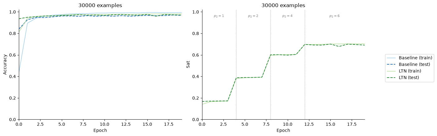
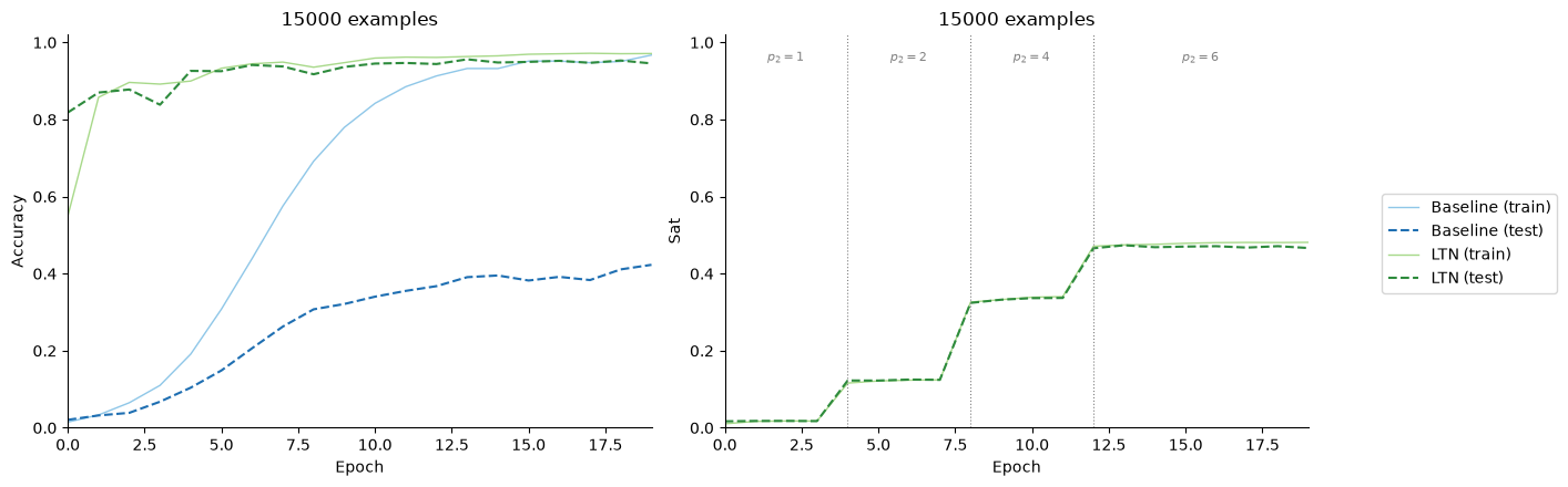
The curves only show the first 20 epochs of the baseline, to line them up with the LTN’s: its final test accuracy, at epoch 30, is 45%.
On adding two digits, the test curves of both approaches almost overlap from start to finish.
On adding two-digit numbers, the baseline overfits: its training accuracy keeps rising, but its test accuracy plateaus. It memorizes the examples without generalizing. The LTN keeps its training and test curves close to each other.
The reason lies in the structure of the problem. The baseline has to predict the sum directly among 199 classes, with 15,000 examples, that is, few examples per class, and extreme sums are very rare. The LTN only learns to tell 10 digits apart, and each training image gives it a signal about one of them; the logical rule then takes care of combining the digits into the sum. It never needs to learn the 199 possible sums.
Satisfaction rises in steps that coincide exactly with the changes of . These jumps need careful reading: for fixed degrees of truth, pMean mechanically increases with , since it gets closer to the maximum. A large part of each jump therefore comes from the change of the measure itself, not from a sudden improvement of the classifier, as confirmed by the accuracy, which does not jump at the same moments. Satisfaction levels are only comparable at equal .
Key takeaways
- An LTN can learn a classifier without any individual label, from a single logical constraint on the sum: the digits are latent variables, linked to the data by the logic alone.
- Diagonal quantification pairs each couple of images with its own result, and guarded quantification injects the rule .
- On adding two digits, LTN and baseline are on par (97%). On adding two-digit numbers, the LTN stays at 95% while the baseline drops to 45%: by breaking the problem down into digits, the logic avoids having to learn 199 classes from few examples.
- The schedule of applies the lesson of part 3: a low at first to spread the gradient, then a higher one once the classifier becomes reliable.
This case study concludes the series. It illustrates LTN’s central idea: logic fixes the form of the reasoning, here “the sum of the digits equals the result”, and the content, recognizing each digit, is learned by gradient descent.
The full notebook for this case study is available in my repository.
Weekly Notes
Every Sunday, I share what I've been learning: papers, ideas, experiments, and questions that stayed with me.
You can unsubscribe at any time with a single click.
Discussion about this post0
Join the discussion
A secure sign-in link will be sent to your email address.
Loading discussion...