
In part 1, we saw how LTN grounds the non-logical symbols (constants, variables, functions and predicates) in tensors. What remains is the logical part of the language: the connectives (, , , ) and the quantifiers (, ). This is what lets us assemble predicates into complete formulas, and obtain a single degree of truth for each formula.
Connectives
Classical connectives cannot be used as they are in LTN: their truth tables are only defined for values in , whereas LTN predicates return degrees of truth anywhere in the interval . LTN therefore replaces them with fuzzy logic operators, defined over the whole continuous interval.
There are several valid families of fuzzy operators (Gödel, product, Łukasiewicz), but they are not equally good for training. Gödel’s /, for instance, only lets the gradient flow to one of its arguments at a time, which can slow down or even block learning. LTN generally recommends the following configuration, where and are two degrees of truth in :
| Connective | Fuzzy operator | Formula |
|---|---|---|
| standard negation | ||
| product t-norm | ||
| product t-conorm (probabilistic sum) | ||
| Reichenbach implication |
This choice is not arbitrary. Unlike /, the product spreads the gradient over both of its arguments at once, which makes it numerically more stable. This trade-off between logical faithfulness and gradient behavior is the subject of part 3.
Notice also that these formulas recover the classical truth tables at the extreme values: with and , the implication equals , just like “true implies false”. In between, they vary continuously.
In LTN, a connective is created with the Connective() constructor, which takes a fuzzy semantics from the ltn.fuzzy_ops module:
import ltn
import torch

Not = ltn.Connective(ltn.fuzzy_ops.NotStandard())
And = ltn.Connective(ltn.fuzzy_ops.AndProd())
Or = ltn.Connective(ltn.fuzzy_ops.OrProbSum())
Implies = ltn.Connective(ltn.fuzzy_ops.ImpliesReichenbach())
Broadcasting
The ltn.Connective wrapper does more than apply the fuzzy formula. It also handles combining subformulas that do not involve the same variables. As we saw in part 1, a formula on alone has shape , and a formula on and has shape . Before applying the operator element-wise, the connective must therefore extend these shapes to make them compatible. This is broadcasting.
To observe it, we define two variables of different sizes, two constants, and a similarity predicate: the same construction as in part 1, which equals 1 when the two points coincide and tends to 0 as they move apart.
x = ltn.Variable('x', torch.randn((10, 2)))  # 10 points in R^2
y = ltn.Variable('y', torch.randn((5, 2)))   # 5 points in R^2

c1 = ltn.Constant(torch.tensor([0.5, 0.0]))
c2 = ltn.Constant(torch.tensor([4.0, 2.0]))

Eq = ltn.Predicate(func=lambda x, y: torch.exp(-torch.norm(x - y, dim=1)))

Eq(c1, c2).valuetensor(0.0178)and are far apart, so their similarity is close to 0. Let’s now try the connectives on concrete cases:
Not(Eq(c1, c2)).valuetensor(0.9822)We do get .
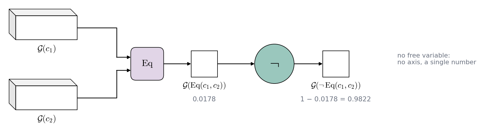
Implies(Eq(c1, c2), Eq(c2, c1)).valuetensor(0.9825)With , the Reichenbach implication gives : an almost false premise makes the implication almost true, as in classical logic.
The next two examples are the most instructive, because they show two different situations with respect to the variables.
And(Eq(x, c1), Eq(x, c2)).shape()torch.Size([10])In And(Eq(x, c1), Eq(x, c2)), only the variable appears in both subformulas. Both results already have the same shape , so no broadcasting is needed: And combines them directly, individual by individual.
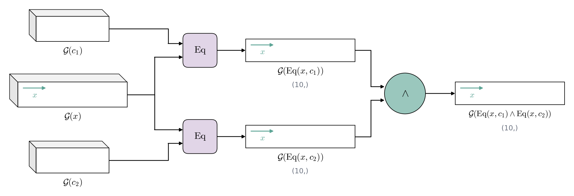
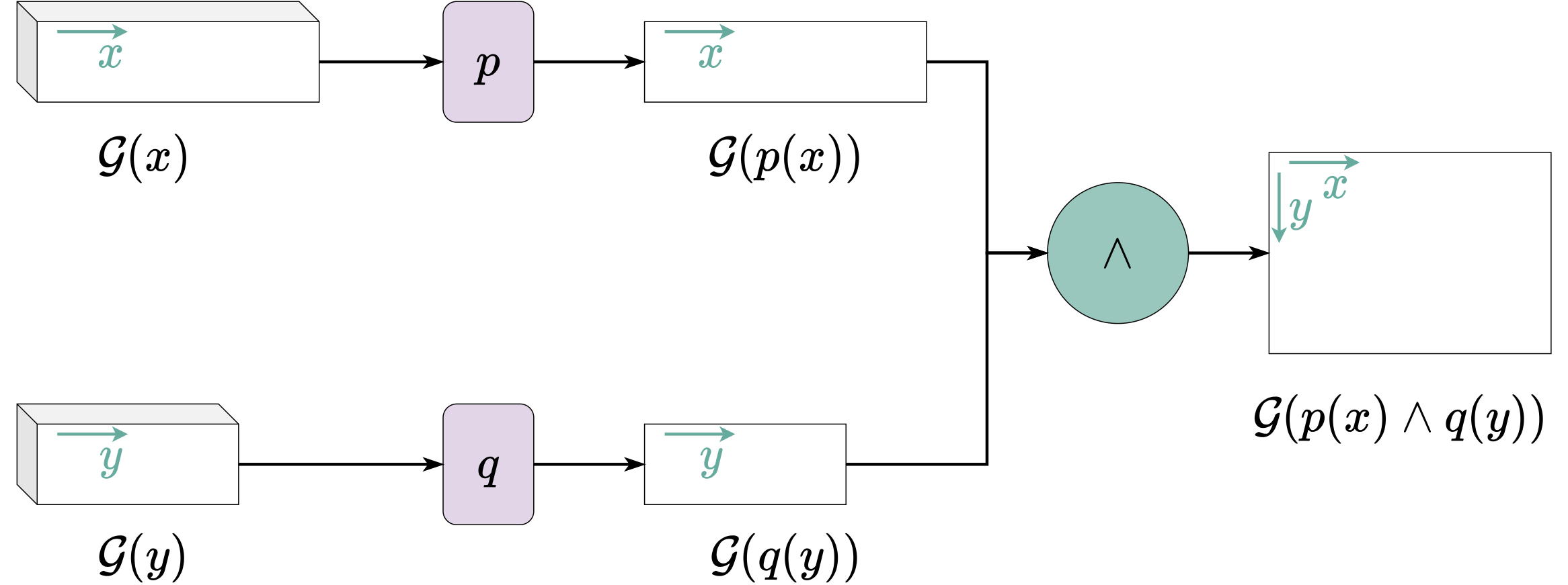
And applied to two subformulas that only depend on : they already have the same shape , and the conjunction combines them individual by individual, with no broadcasting.Or(Eq(x, c1), Eq(x, y)).shape()torch.Size([10, 5])In Or(Eq(x, c1), Eq(x, y)), the situation is different. Eq(x, c1) only depends on and has shape , while Eq(x, y) depends on both and and has shape : an evaluation over two variables produces every combination. The connective detects this mismatch and extends the first result along the missing axis, that of , by repeating each value for the 5 individuals of . It then applies Or element-wise, hence the final shape .
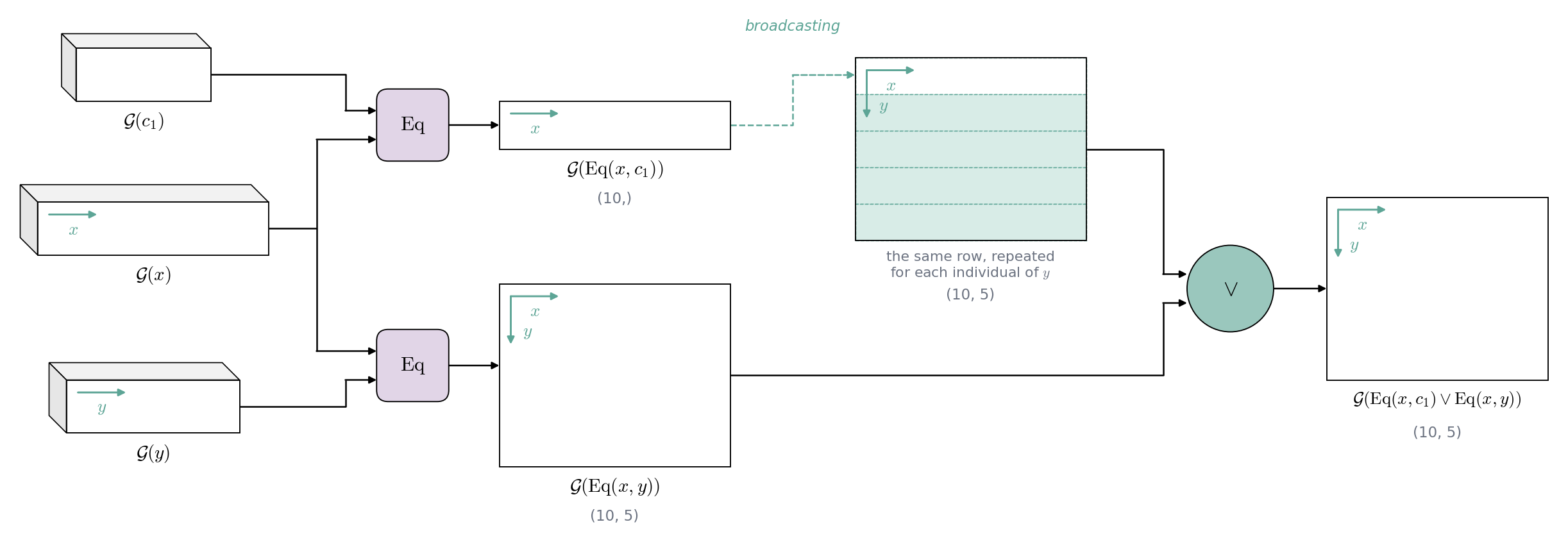
Or applied to , of shape , and to , of shape : the first result is first copied along the axis of , then the disjunction is applied entry by entry.The figure from the paper shows the same mechanism in the general case of two subformulas that each involve a different variable:
Like predicates and functions, connectives return LTNObjects: we read the result with .value and its shape with shape().
Quantifiers
Quantifiers cannot be used in their classical form either. and assume that a property is checked over an entire domain, whereas in LTN a variable only represents a finite batch of individuals, with continuous degrees of truth. LTN therefore replaces them with aggregation operators, which condense the degrees of truth of a batch into a single value.
For a list of degrees of truth in , the two recommended operators are:
- for , the generalized mean (
pMean):
- for , the generalized mean of the deviations from truth (
pMeanError):
These formulas are not chosen at random: pMean approximates the maximum and pMeanError the minimum. That is exactly the spirit of , for which a single individual satisfying the property is enough, and of , for which the worst case is what counts. We will prove it a little further down.
A quantifier is created with the Quantifier() constructor, which takes an aggregation semantics and the type of quantification: "e" for existential, "f" for universal.
Forall = ltn.Quantifier(ltn.fuzzy_ops.AggregPMeanError(p=2), quantifier="f")
Exists = ltn.Quantifier(ltn.fuzzy_ops.AggregPMean(p=2), quantifier="e")
Quantifying means aggregating along an axis
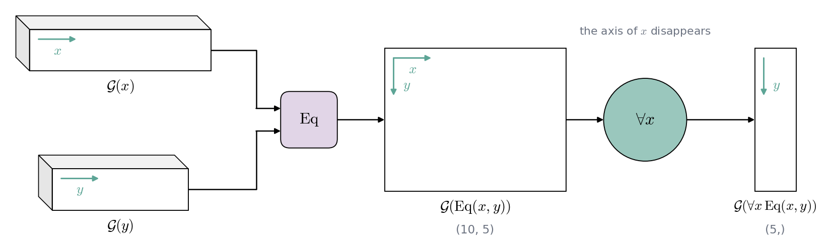
The ltn.Quantifier wrapper itself picks the dimensions to aggregate, based on the variables passed to it. Quantifying over a variable amounts to applying the aggregator along that variable’s axis, which makes that axis disappear from the result. This is where the variable labels seen in part 1 really pay off.
x = ltn.Variable('x', torch.randn((10, 2)))  # 10 points in R^2
y = ltn.Variable('y', torch.randn((5, 2)))   # 5 points in R^2

Eq = ltn.Predicate(func=lambda x, y: torch.exp(-torch.norm(x - y, dim=1)))

Eq(x, y).shape()
torch.Size([10, 5])Let’s quantify over alone:
Forall(x, Eq(x, y)).shape()torch.Size([5])The axis of is gone, only that of remains. The result is still a function of : for each of the 5 individuals of , it tells to what degree the property holds for every .
When the quantification covers both variables, both axes disappear and we get a scalar, a single degree of satisfaction for the whole formula:
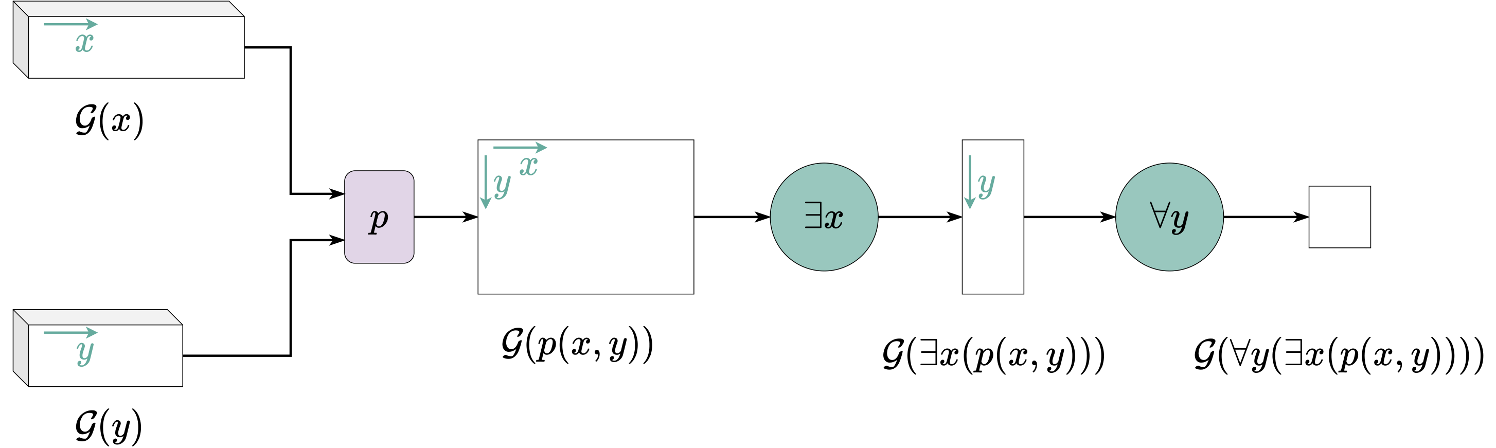
Forall([x, y], Eq(x, y)).valuetensor(0.1521)Exists([x, y], Eq(x, y)).valuetensor(0.2211)Forall(x, Exists(y, Eq(x, y))).valuetensor(0.1846)The last example nests two quantifiers: “for every , there is a similar ”. Exists(y, …) first removes the axis of and leaves a vector of shape , which Forall(x, …) then reduces to a scalar.
A point of syntax to remember: a single variable is passed to the quantifier directly, while several variables must be grouped in a list, like [x, y].
Why pMean tends to the maximum, and pMeanError to the minimum
We claimed that pMean approximates the maximum and pMeanError the minimum. Let’s prove it.
pMean tends to the maximum. We want to show that, for :
Let . The case is trivial (all the are zero and pMean equals 0); we therefore assume , which lets us factor it out:
Let , which lies in since . Two cases arise:
- for an index that achieves the maximum, , so for every ;
- for any other index, , and a number strictly less than 1 raised to an ever-growing power tends to 0.
Writing for the number of indices that achieve the maximum (usually , but ties are possible):
What remains is the -th root. Since is a strictly positive constant, we use the classical result for every : just write and note that . Hence:
pMeanError tends to the minimum. We want to show that:
The trick is to apply the previous result not to the , but to their complements , which are also in :
Now, .
Justification
Let . For every , , so : is an upper bound of the family, and .
The minimum of a finite family is attained: there is an such that , so is one of the terms of the family. Since the maximum is greater than or equal to every term, .
The two inequalities give the equality.
We conclude:
The role of p
pMean is thus a smoothed maximum: for , it is a plain mean, and as , it tends to the strict maximum. Likewise, pMeanError is a smoothed minimum, which goes from the mean () to the strict minimum ().
The parameter actually sets a trade-off between logical faithfulness and tolerance to the hard cases of the batch.
When is high, pMeanError gets close to the true minimum, and recovers its strict meaning: a single individual with a low degree of truth is enough to make the result drop, as we expect from a rigorous “for all”. This is faithful, but demanding: to get a high score, every individual without exception must have a high degree of truth. Symmetrically, pMean gets close to the true maximum, and becomes easy to satisfy again: one good individual is enough.
When gets close to 1, both operators get close to a mean in which each individual weighs about the same. Extreme cases then stop dominating: a very bad individual can be offset by several good ones, and vice versa. This compensation makes more tolerant (one failing individual is no longer enough to bring everything down) and more demanding (a single good individual is no longer enough). It is a deliberate departure from the strict logical semantics, useful in practice for absorbing noise in the data or for spreading the gradient more evenly during training.
The choice of therefore depends on the goal: a high for a formula that must stay strict and tolerate no exception, a close to 1 for a formula that must be robust to noisy data or outliers. This choice also has major consequences for training, which we will see in part 3.
can be set when the operator is created, or changed at each call:
Forall(x, Eq(x, c1), p=2).valuetensor(0.1942)Forall(x, Eq(x, c1), p=10).valuetensor(0.1232)Exists(x, Eq(x, c1), p=2).valuetensor(0.3085)Exists(x, Eq(x, c1), p=10).valuetensor(0.6013)When goes from 2 to 10, drops (from 0.19 to 0.12) because it gets closer to the worst individual, and rises (from 0.31 to 0.60) because it gets closer to the best one.
Diagonal quantification
So far, evaluating a predicate on two variables always produced every combination of their individuals. That is not always what we want. In a supervised dataset, each data point has its own label : we want to evaluate the predicate on the pairs , , and so on, never on crossed combinations like , which make no sense.
This is what ltn.diag does: instead of crossing every combination, it only keeps the pairs in one-to-one correspondence, like a Python zip rather than two nested loops. This requires the variables to have the same number of individuals.
Consider the following example:
- the variable holds 100 individuals in ;
- the variable holds the 100 corresponding labels, one-hot encoded (3 classes);
- each pair is an example of the dataset;
- the classifier returns a degree of confidence in that sample matches label .
# Random values for illustration; in practice, they would come from a dataset
samples = torch.randn((100, 2, 2))         # 100 values in R^{2x2}
labels = torch.randint(0, 3, size=(100,))  # the label (class 0, 1 or 2) of each sample
onehot_labels = torch.nn.functional.one_hot(labels, num_classes=3)

x = ltn.Variable("x", samples)
l = ltn.Variable("l", onehot_labels)

class ModelC(torch.nn.Module):
    def __init__(self):
        super().__init__()
        self.elu = torch.nn.ELU()
        self.softmax = torch.nn.Softmax(dim=1)
        self.dense1 = torch.nn.Linear(4, 5)
        self.dense2 = torch.nn.Linear(5, 3)

    def forward(self, x, l):
        x = torch.flatten(x, start_dim=1)   # the 2 x 2 matrix becomes a vector of size 4
        x = self.elu(self.dense1(x))
        x = self.softmax(self.dense2(x))    # one probability per class
        return torch.sum(x * l, dim=1)      # keep the probability of class l

C = ltn.Predicate(ModelC())
The last line of forward deserves an explanation. If the network outputs for a sample whose label is , the element-wise product followed by the sum gives : the probability the network assigns to the correct class.
Without ltn.diag, C(x, l) evaluates the combinations. Let’s shrink the example to 4 individuals to see the problem: of the 16 pairs produced, only the 4 on the diagonal, to , are real examples. All the others ask a question we never meant to ask, such as “does sample have the label of example 1?”.
ltn.diag(x, l) keeps only the 100 matching pairs: the shape of the result goes from to .
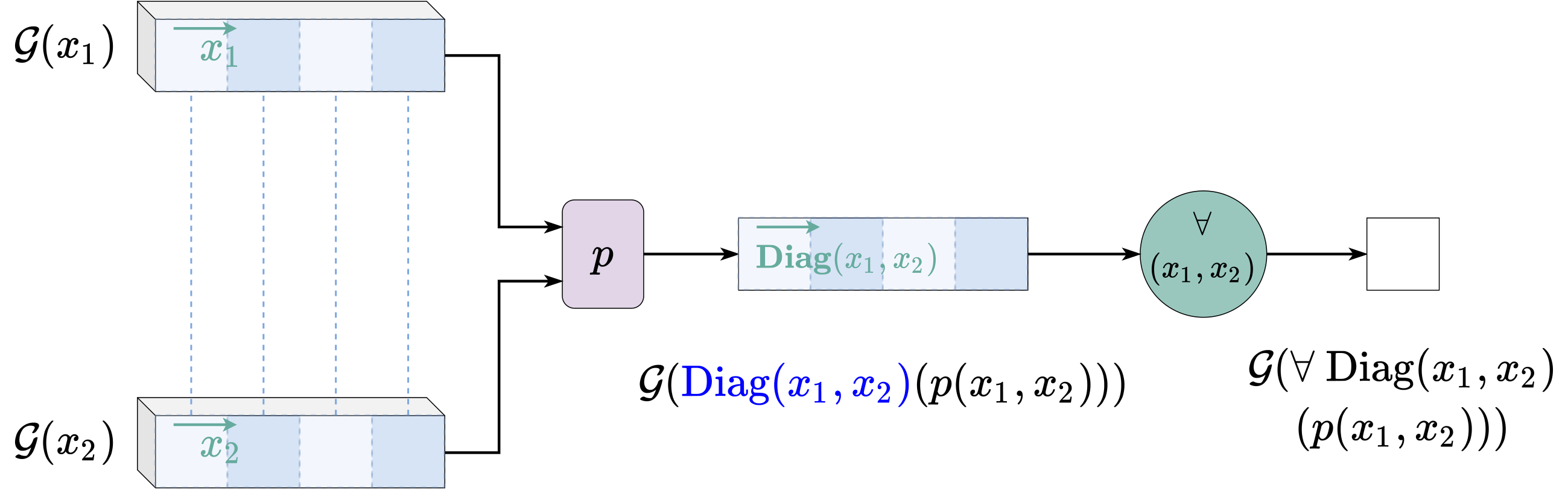
Once again, the mechanism relies on variable labels: ltn.diag temporarily gives and the same label, prefixed with diag_. Since LTN relies on labels to decide whether two variables are crossed or traversed together, sharing the same label is enough to switch from the full cross product to one-to-one correspondence. ltn.undiag restores the original labels.
print(C(x, l).shape())  # the 100 x 100 combinations
ltn.diag(x, l)          # switch on one-to-one correspondence
print(C(x, l).shape())  # the 100 matching pairs
print(x.free_vars)
print(l.free_vars)
ltn.undiag(x, l)        # restore the normal behavior
print(C(x, l).shape())  # the 100 x 100 combinations again
torch.Size([100, 100])
torch.Size([100])
['diag_x_l']
['diag_x_l']
torch.Size([100, 100])In practice, ltn.diag is used right before a quantifier. Every quantifier automatically calls ltn.undiag once the aggregation is done, so the variables recover their normal behavior outside the formula.
x, l = ltn.diag(x, l)
print(x.free_vars)
print(l.free_vars)
print(Forall([x, l], C(x, l)).value)  # aggregates only over the 100 matching pairs
print(x.free_vars)                    # undiag was called automatically
print(l.free_vars)
['diag_x_l']
['diag_x_l']
tensor(0.3384, grad_fn=<RsubBackward1>)
['x']
['l']asks exactly the question of a supervised classification problem: to what degree does the model assign good confidence to each example paired with its true label? Since the network is not trained, the score is low.
Guarded quantifiers
Sometimes we want to quantify not over all the individuals of a variable, but only over those that satisfy a condition. This condition is not a continuous degree of truth like an LTN predicate: it is a boolean mask, strictly 0 or 1, used only to select which individuals take part in the aggregation.
Let be a masking function that returns a boolean for each element of the domain. We can then write:
- : “every that satisfies also satisfies ”;
- : “there is an that satisfies and also satisfies ”.
The mask can depend on other variables of the formula: is a valid statement, where the condition on depends on .
Take an example stating that there is a distance below which all pairs of points are similar:
is the similarity predicate used so far, and computes the Euclidean distance between two points.
Eq = ltn.Predicate(func=lambda x, y: torch.exp(-torch.norm(x - y, dim=1)))

points = torch.rand((50, 2))  # 50 points in [0,1]^2
x = ltn.Variable("x", points)
y = ltn.Variable("y", points)
d = ltn.Variable("d", torch.tensor([.1, .2, .3, .4, .5, .6, .7, .8, .9]))
A guarded quantifier takes two extra arguments: cond_vars, the list of variables the condition depends on, and cond_fn, the function that computes the mask from those variables.
dist = lambda x, y: torch.unsqueeze(torch.norm(x.value - y.value, dim=1), 1)

Exists(d,
      Forall([x, y],
            Eq(x, y),
            cond_vars=[x, y, d],
            cond_fn=lambda x, y, d: dist(x, y) < d.value
            )).value
tensor(0.7599, dtype=torch.float64)Here, cond_vars=[x, y, d] says that the condition depends on , and , and cond_fn checks, for each combination, whether the distance between and is below the threshold . LTN computes over every combination, computes the mask in parallel, then only aggregates the values for which the mask is true. Pairs that are too far apart are simply left out.
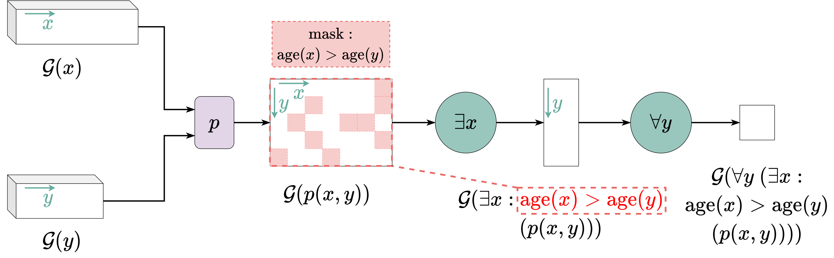
This is especially useful for learning: the gradient then only flows through the part of the domain that satisfies the condition, instead of being diluted over combinations that make no sense for the rule.
Key takeaways
- Connectives become differentiable fuzzy operators. The recommended configuration: standard negation, product, probabilistic sum and Reichenbach implication.
- A connective automatically broadcasts subformulas that do not involve the same variables.
- Quantifiers become aggregations along the axis of the quantified variable:
pMeanErrorfor , a smoothed minimum, andpMeanfor , a smoothed maximum. - The parameter sets the trade-off between logical faithfulness (large ) and tolerance to noise (small ).
ltn.diagreplaces the full cross product with one-to-one correspondence, which is essential for (data, label) pairs.- Guarded quantifiers restrict the aggregation to the individuals that satisfy a boolean mask.
We can now evaluate any formula. But for a network to learn to satisfy these formulas, their gradient must behave well, and that is not the case for every operator. In part 3, we will look at the gradient pitfalls and at the “stable product” configuration that avoids them.
The full notebook for this part is available in my repository.
Weekly Notes
Every Sunday, I share what I've been learning: papers, ideas, experiments, and questions that stayed with me.
You can unsubscribe at any time with a single click.
Discussion about this post0
Join the discussion
A secure sign-in link will be sent to your email address.
Loading discussion...