
In the first three parts, we learned to build LTN objects and evaluate formulas, but never to make a predicate improve. That is the subject of this last part: learning symbols of the language (predicates, functions, constants) by using the satisfaction of a knowledge base as the training objective.
A knowledge base is simply a set of formulas we want to hold at the same time. Satisfying it does not mean making each formula strictly true, as in classical logic, but finding the parameters that bring each formula’s degree of truth as close as possible to 1. It is a continuous optimization problem, just like minimizing a loss function, except that we maximize a degree of logical satisfaction rather than closeness to labels.
During training, what changes are the weights of the trainable predicates and functions (the neural networks we have built so far), and possibly the values of trainable constants. The logical structure of the formulas stays fixed.
A proximity classification problem
The domain is the square : points in the plane whose two coordinates are between 0 and 4. We have 19 points and want to guess their class. Only two of them are labeled: point , of class , and point , of class . The other 17 have no label.
With two labeled examples, a classifier trained in a purely supervised way would learn nothing useful. The idea is to make up for the lack of data with prior knowledge about the problem, expressed as two assumptions:
- classes and are mutually exclusive: a point cannot belong to both;
- two nearby points should have the same label.
The second assumption will do most of the work. It echoes the principle of k nearest neighbors: a point close to probably belongs to the same class as . We are going to turn it into a logical rule, which will let the model classify every point from the two labeled examples alone, without ever receiving the label of the other 17.
import torch
import numpy as np
import ltn
import matplotlib.pyplot as plt

points = np.array(
        [[0.4,0.3], [1.2,0.3], [2.2,1.3], [1.7,1.0], [0.5,0.5], [0.3, 1.5], [1.3, 1.1], [0.9, 1.7],
        [3.4,3.3], [3.2,3.3], [3.2,2.3], [2.7,2.0], [3.5,3.5], [3.3, 2.5], [3.3, 1.1], [1.9, 3.7], [1.3, 3.5],
        [3.3, 1.1],[3.9, 3.7]])
point_a = [3.3, 2.5]
point_b = [1.3, 1.1]
fig, ax = plt.subplots()
ax.set_xlim(0, 4)
ax.set_ylim(0, 4)
ax.scatter(points[:,0], points[:,1], color="black", label="unknown")
ax.scatter(point_a[0], point_a[1], color="blue", label="a")
ax.scatter(point_b[0], point_b[1], color="red", label="b")
ax.set_title("Dataset of individuals")
plt.legend();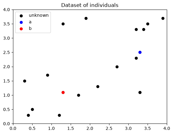
The knowledge base
We define a membership predicate , where is a point and a one-hot encoded label: for class , for class . answers the question “to what degree does point belong to class ?”.
is a small multilayer perceptron. Its last layer uses a softmax rather than a sigmoid, and this choice directly encodes the first assumption. A sigmoid would evaluate each class independently; the softmax spreads a total probability mass of 1 across the classes, which makes them mutually exclusive.
The knowledge base contains three formulas:
where:
- and are the two labeled points, and , the one-hot labels of and ;
- and are variables that range over all the points;
- is a variable that ranges over the two labels;
- measures the similarity between two points: , the construction already met in the previous parts.
The first two formulas require to be recognized as class , and as class . The third encodes the proximity assumption: for every pair of points and for each label, if the two points are similar, they must get the same verdict for that label. This is what the equivalence inside the implication expresses.
The goal is to learn so as to maximize the overall satisfaction of . Writing for the weights of the network that implements , we are looking for:
where aggregates the degrees of truth of all the formulas of into a single value. We will come back to it a little further down.
Let’s first define the predicates, with the same names as in the mathematical formulation:
# Predicate C
class ModelC(torch.nn.Module):
    def __init__(self):
        super().__init__()
        self.elu = torch.nn.ELU()
        self.softmax = torch.nn.Softmax(dim=1)
        self.dense1 = torch.nn.Linear(2, 5)
        self.dense2 = torch.nn.Linear(5, 5)
        self.dense3 = torch.nn.Linear(5, 2)

    def forward(self, x, l):
        """x: a point, l: a one-hot label"""
        x = self.elu(self.dense1(x))
        x = self.elu(self.dense2(x))
        prob = self.softmax(self.dense3(x))
        return torch.sum(prob * l, dim=1)

C = ltn.Predicate(ModelC())

# Predicate Sim
Sim = ltn.Predicate(func=lambda u, v: torch.exp(-1. * torch.sqrt(torch.sum(torch.square(u - v), dim=1))))
Then the variables and constants: and range over the 19 points, and are the two labeled points, and their labels, and ranges over the two possible labels.
x1 = ltn.Variable("x1", torch.tensor(points))
x2 = ltn.Variable("x2", torch.tensor(points))
a = ltn.Constant(torch.tensor([3.3, 2.5]))
b = ltn.Constant(torch.tensor([1.3, 1.1]))
l_a = ltn.Constant(torch.tensor([1, 0]))
l_b = ltn.Constant(torch.tensor([0, 1]))
l = ltn.Variable("l", torch.tensor([[1, 0], [0, 1]]))
Let’s visualize the similarity between each point and , as computed by : the thicker and more opaque the line linking a point to , the more similar they are.
similarities_to_a = Sim(x1, a).value
fig, ax = plt.subplots()
ax.set_xlim(0, 4)
ax.set_ylim(0, 4)
ax.scatter(points[:,0], points[:,1], color="black")
ax.scatter(a.value[0], a.value[1], color="blue")
ax.set_title("Illustrating the similarities of each point to a")
for i, sim_to_a in enumerate(similarities_to_a):
    plt.plot([points[i,0], a.value[0]], [points[i,1],a.value[1]], alpha=float(sim_to_a.numpy()), color="blue")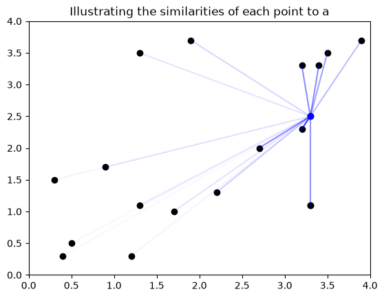
For the connectives, we use the product configuration seen in part 3. A new operator appears: equivalence . LTN does not implement it as a standalone operator, but builds it from two known operators, following the classical equivalence . ltn.fuzzy_ops.Equiv takes the t-norm and the implication to use for this construction.
Not = ltn.Connective(ltn.fuzzy_ops.NotStandard())
And = ltn.Connective(ltn.fuzzy_ops.AndProd())
Or = ltn.Connective(ltn.fuzzy_ops.OrProbSum())
Implies = ltn.Connective(ltn.fuzzy_ops.ImpliesReichenbach())
Equiv = ltn.Connective(ltn.fuzzy_ops.Equiv(ltn.fuzzy_ops.AndProd(), ltn.fuzzy_ops.ImpliesReichenbach()))
Forall = ltn.Quantifier(ltn.fuzzy_ops.AggregPMeanError(p=2), quantifier="f")
Exists = ltn.Quantifier(ltn.fuzzy_ops.AggregPMean(p=6), quantifier="e")
From closed formulas to a loss function
When contains several formulas, their degrees of truth must be aggregated into a single value: that is the role of . It only applies to closed formulas, that is, formulas with no free variable: all their variables have been captured by a quantifier. If a formula still contained a free variable, its degree of truth would not be a single number but a tensor of values, one per value of the variable, and would not know which one to keep.
A few examples to pin down this criterion:
- has two free variables: it is not closed, and evaluating it gives a matrix.
- is not closed either: remains free, and the result is a vector, one value per .
- is closed: evaluating it gives a scalar.
- is closed too. All that matters is that every variable is quantified, not the order or the type of the quantifiers.
In our base, and are closed from the start, since they only contain constants: there is nothing to quantify. The third only becomes closed thanks to the that captures its three variables.
In LTN, is available through ltn.fuzzy_ops.SatAgg, whose constructor takes an aggregation operator. Here again we recommend pMeanError, the same as for , and it is the default. plays the same role as for quantifiers: the lower it is, the closer the aggregation gets to a mean of the formulas; the higher it is, the closer it gets to the worst formula of . SatAgg directly accepts LTNObjects: no need to go through .value.
Finally, we want to maximize satisfaction, whereas PyTorch optimizers minimize a loss. We therefore define the loss as : minimizing it is exactly the same as maximizing satisfaction.
A worked example by hand
Before starting training, let’s follow the computation of the third formula on a case small enough to be done by hand. We use the product configuration:
- Reichenbach implication: ;
- equivalence: , the product of the two implications.
In these formulas, and are scalars: individual degrees of truth in .
The data
We take 3 points instead of 19:
and range independently over this same domain, so any formula is computed over the Cartesian product, a grid indexed by .
Step 1: Sim(x1, x2)
The matrix is symmetric, and its diagonal is 1 since each point is identical to itself. and are very close, is far from both.
Step 2: C(x, l), the confidence predicate
is a function of a single point and a label. Suppose the network, not yet trained, gives the following confidences (one row per point, one column per label):
and range over the same domain with the same predicate: and are the same function, evaluated at different indices ( for , for ). For a fixed label, we therefore extract a vector indexed by the points:
Thanks to the softmax, the two columns sum to 1: element-wise.
Step 3: Equiv(C(x1, l), C(x2, l))
and are two values of the same vector, taken at two indices. For , with :
The matrix is symmetric, since by construction:
Why is ? Since , we have . Now:
so:
The two matrices have exactly the same 9 values, for an algebraic reason and not by coincidence.
Step 4: Implies(Sim(x1, x2), Equiv(C(x1, l), C(x2, l)))
and are indexed by the same grid, since both come from the grounding of and . The implication is therefore computed entry by entry:
The rule can be read directly: when two points are far apart ( close to 0), the implication is almost true whatever their disagreement, because the rule says nothing about them. When they are close, the agreement of their confidences decides.
Reading one entry
Each entry answers a precise question, fixed by the three indices: taking , and the label , to what degree does the axiom “if they are similar, they get the same confidence for this label” hold?
Take :
- We instantiate , and .
- : the two points are very close.
- : the network gives 90% confidence for class , but only 50% to . The two verdicts disagree.
- .
A value of , far from 1, signals a violation of the axiom: two nearby points should get close confidences for class . This kind of entry is what will produce a strong gradient signal, pushing the network to bring and closer.
Step 5: the ∀ quantifier
Forall([x1, x2, l], …) aggregates the entries with pMeanError and :
| entries per label | ||||
|---|---|---|---|---|
| 1 | ||||
| 1 | ||||
| 1 | ||||
| , | 2 | |||
| , | 2 | |||
| , | 2 |
For one label, the sum is , and since , it is counted twice:
Notice the diagonal. One might think that comparing a point with itself is trivially true, but that is not the case in fuzzy logic: only equals 1 when is 0 or 1. For , whose confidence is , entry is only , and it is even the worst entry in the table. The training code below aggregates over all pairs, diagonal included: these entries therefore push the network toward clear-cut verdicts, close to 0 or 1, rather than undecided confidences.
The loss
The loss finally combines the three formulas of :
Why compare every pair?
One could imagine a simpler rule: compare each unknown point with and only, and infer its class from that, like a nearest-neighbor algorithm with two reference neighbors:
This rule would only light up the points close enough to the two lamps and : a point too far away would stay in the dark, even if surrounded by points that are already well lit. The rule of compares every pair: each lit point in turn lights up its neighbors, and the light spreads from one end of the point cloud to the other, even very far from and , as long as there is a path of successive proximities.
This is what justifies the computational cost, pairs instead of : it is not needless overhead, it is what lets information flow through the whole proximity graph.
Training
Each iteration computes the degrees of truth of the three formulas of (forward pass), then adjusts the weights of by backpropagation to reduce the loss (backward pass).
# by default, SatAgg uses pMeanError
sat_agg = ltn.fuzzy_ops.SatAgg()

# we learn the parameters of the predicate C
optimizer = torch.optim.Adam(C.parameters(), lr=0.001)

for epoch in range(2000):
    optimizer.zero_grad()
    loss = 1. - sat_agg(
        C(a, l_a),
        C(b, l_b),
        Forall([x1, x2, l], Implies(Sim(x1, x2), Equiv(C(x1, l), C(x2, l))))
    )
    loss.backward()
    optimizer.step()
    if epoch%200 == 0:
        print("Epoch %d: Sat Level %.3f "%(epoch, 1 - loss.item()))
print("Training finished at Epoch %d with Sat Level %.3f" %(epoch, 1 - loss.item()))
Epoch 0: Sat Level 0.487
Epoch 200: Sat Level 0.726
Epoch 400: Sat Level 0.935
Epoch 600: Sat Level 0.955
Epoch 800: Sat Level 0.958
Epoch 1000: Sat Level 0.959
Epoch 1200: Sat Level 0.959
Epoch 1400: Sat Level 0.959
Epoch 1600: Sat Level 0.959
Epoch 1800: Sat Level 0.959
Training finished at Epoch 1999 with Sat Level 0.960Satisfaction goes from 0.49 to 0.96 in a few hundred iterations. The system has learned to recognize the points close to as class , and those close to as class , relying only on the rules of the knowledge base, without ever receiving the label of the other 17 points.
The two plots below show it: the lighter the color, the more is satisfied. On the left, ; on the right, .
fig = plt.figure(figsize=(10, 3))

fig.add_subplot(1, 2, 1)
plt.scatter(x1.value[:, 0], x1.value[:, 1], c=C(x1, l_a).value.detach().numpy(), vmin=0, vmax=1)
plt.scatter(a.value[0], a.value[1], marker="x", color="red", s=100, label="a")
plt.scatter(b.value[0], b.value[1], marker="x", color="blue", s=100, label="b")
plt.title("C(x,l_a)")
plt.legend()
plt.colorbar()

fig.add_subplot(1, 2, 2)
plt.scatter(x1.value[:, 0], x1.value[:, 1], c=C(x1, l_b).value.detach().numpy(), vmin=0, vmax=1)
plt.scatter(a.value[0], a.value[1], marker="x", color="red", s=100, label="a")
plt.scatter(b.value[0], b.value[1], marker="x", color="blue", s=100, label="b")
plt.title("C(x,l_b)")
plt.legend()
plt.colorbar()

plt.show();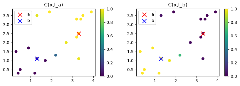
We can see the propagation at work: the points at the top left, around , are almost as far from as from , and yet they are classified as , thanks to the chain of neighbors linking them to . Only the point , between the two groups, gets a less clear-cut verdict.
Working in mini-batches
In most learning tasks, we work in batches rather than with the whole dataset at each iteration, especially when it is too large to be processed at once.
In LTN, this requires no special mechanism: we simply reground the variables with different values at each step. In PyTorch, these values usually come from a DataLoader, which splits the dataset and hands out the subsets over the iterations.
Let’s take the same problem with 10,000 random points. and are deliberately placed fairly far apart, to keep the example readable.
r1 = 0
r2 = 4
points = (r1 - r2) * torch.rand((10000, 2)) + r2
points[-1] = torch.tensor([3., 3.])
points[-2] = torch.tensor([1., 1.])
points_a = torch.tensor([3., 3.])
points_b = torch.tensor([1., 1.])
a = ltn.Constant(torch.tensor([3., 3.]))
b = ltn.Constant(torch.tensor([1., 1.]))

fig, ax = plt.subplots()
ax.set_xlim(0, 4)
ax.set_ylim(0, 4)
ax.scatter(points[:,0], points[:,1], color="black", label="unknown")
ax.scatter(points_a[0], points_a[1], color="blue", label="a")
ax.scatter(points_b[0], points_b[1], color="red", label="b")
ax.set_title("Dataset of individuals")
plt.legend();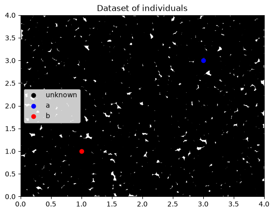
We define a data loader that returns a batch of points at each iteration, with a batch size and optional shuffling at each epoch. The training principle stays the same: the same three formulas, aggregated by SatAgg, then backpropagation. The only difference is that and now hold 512 different points at each iteration.
# redefine C to reset its weights
C = ltn.Predicate(ModelC())

# data loader that creates the batches
class DataLoader:
    def __init__(self,
                 dataset,
                 batch_size=1,
                 shuffle=True):
        self.data = dataset
        self.batch_size = batch_size
        self.shuffle = shuffle

    def __len__(self):
        return int(np.ceil(self.data.shape[0] / self.batch_size))

    def __iter__(self):
        n = self.data.shape[0]
        idxlist = list(range(n))
        if self.shuffle:
            np.random.shuffle(idxlist)

        for _, start_idx in enumerate(range(0, n, self.batch_size)):
            end_idx = min(start_idx + self.batch_size, n)
            batch_points = self.data[idxlist[start_idx:end_idx]]

            yield batch_points

train_loader = DataLoader(points, 512)

sat_agg = ltn.fuzzy_ops.SatAgg()
optimizer = torch.optim.Adam(C.parameters(), lr=0.001)

for epoch in range(100):
    for (batch_idx, (batch_points)) in enumerate(train_loader):
        x1 = ltn.Variable("x1", batch_points)  # reground the variables
        x2 = ltn.Variable("x2", batch_points)  # with the current batch
        optimizer.zero_grad()
        loss = 1. - sat_agg(
            C(a, l_a),
            C(b, l_b),
            Forall([x1, x2, l], Implies(Sim(x1, x2), Equiv(C(x1, l), C(x2, l))))
        )
        loss.backward()
        optimizer.step()
    if epoch%10 == 0:
        print("Epoch %d: Sat Level %.3f "%(epoch, 1 - loss.item()))

print("Training finished at Epoch %d with Sat Level %.3f" %(epoch, 1 - loss.item()))
Epoch 0: Sat Level 0.670
Epoch 10: Sat Level 0.890
Epoch 20: Sat Level 0.943
Epoch 30: Sat Level 0.947
Epoch 40: Sat Level 0.948
Epoch 50: Sat Level 0.953
Epoch 60: Sat Level 0.946
Epoch 70: Sat Level 0.948
Epoch 80: Sat Level 0.952
Epoch 90: Sat Level 0.951
Training finished at Epoch 99 with Sat Level 0.951After about twenty epochs, satisfaction is already above 0.94, despite the size of the dataset and the fact that the model only sees mini-batches. It then oscillates slightly, since each batch is different. Let’s draw the same plots on the 10,000 points:
x1 = ltn.Variable("x1", points)
x2 = ltn.Variable("x2", points)
fig = plt.figure(figsize=(10, 3))
fig.add_subplot(1, 2, 1)
plt.scatter(x1.value[:, 0], x1.value[:, 1], c=C(x1, l_a).value.detach().numpy(), vmin=0, vmax=1)
plt.title("C(x,l_a)")
plt.colorbar()
fig.add_subplot(1, 2, 2)
plt.scatter(x1.value[:, 0], x1.value[:, 1], c=C(x1, l_b).value.detach().numpy(), vmin=0, vmax=1)
plt.title("C(x,l_b)")
plt.colorbar()
plt.show();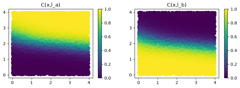
LTN has indeed learned to separate the two classes. The points in the middle band remain harder to classify, which matches intuition: their distances to and are comparable, and LTN then has no clear proximity information to decide.
Key takeaways
- A knowledge base is a set of closed formulas; learning it means finding the parameters that maximize their satisfaction.
SatAggaggregates the satisfaction of the formulas into a single value, and the loss is .- Only the weights of trainable predicates, functions and constants change; the logical structure stays fixed.
- Prior knowledge, such as “two nearby points have the same class”, makes it possible to learn from very few labels, because information spreads through every pair.
- Working in mini-batches simply means regrounding the variables at each iteration.
This part wraps up the presentation of LTN’s mechanisms. The same principle, logical knowledge turned into a loss function, goes much further: in the case study of part 5, an LTN learns to recognize handwritten digits without ever seeing their labels, from the sum of two digits alone.
The full notebook for this part is available in my repository.
Weekly Notes
Every Sunday, I share what I've been learning: papers, ideas, experiments, and questions that stayed with me.
You can unsubscribe at any time with a single click.
Discussion about this post0
Join the discussion
A secure sign-in link will be sent to your email address.
Loading discussion...