

Introduction
Anomaly detection in multivariate time series is not just about flagging whether something went wrong; it is also about pinpointing when the anomaly occurred and which variables caused it. This fine-grained localization is critical when monitoring complex systems featuring dozens or hundreds of concurrent sensors.
However, having a sequence-level label indicating that a full temporal window is abnormal does not tell us the exact timestamps or the specific metrics responsible. Gathering point-wise and variable-wise labels is notoriously labor-intensive and costly. Multiple Instance Learning (MIL) offers an appealing framework for this weakly supervised setting: models are trained using only coarse sequence-level annotations while learning to localize anomalies at finer granularities.
Against this backdrop, Jang and Kwon introduced TAIL-MIL (Time-Aware and Instance-Learnable Multiple Instance Learning for Multivariate Time Series Anomaly Detection), an architecture designed to detect anomalies across multiple levels of abstraction in multivariate time series. The authors formulate time series data as a two-dimensional hierarchical structure: a full temporal window, called a Time-Aware Bag (TAB), consists of multiple time-step instances (Time-Point Instances in Multivariate data, TPIM), each comprising variable-level instances (Variate Instances in TPIM, VI-TPIM).
The goal is to design a unified model that predicts whether a temporal window is abnormal, pinpoints the timestamps involved, and identifies the anomalous variables. To achieve this, the authors establish three core research objectives:
- R1 — Model instance relationships: The attention mechanism must take into account interactions across VI-TPIMs belonging to different TPIMs to fully capture temporal dependencies.
- R2 — Build bag-level predictions directly from instance predictions: Bag-level (TAB) decisions must be derived directly from fine-grained instance predictions, unifying global anomaly detection and local fault localization.
- R3 — Preserve local feature integrity: Individual predictions must be computed from original, uncorrupted instance embeddings, without being distorted by context injected from other time steps.
To satisfy these three requirements, TAIL-MIL couples two distinct attention modules — T-Attention and V-Attention — with a bottom-up hierarchical aggregation scheme.
Hierarchical Problem Formulation
Consider a temporal window (TAB) , where each represents the -th TPIM (time step).
Each TPIM is composed of variables (the VI-TPIMs):
where denotes the value of variable at time step .
The model must jointly learn:
- Which specific variable-time cell is abnormal.
- Which time step is abnormal.
- Whether the overall bag (TAB) is abnormal.
The Underlying Boolean Logic
Ideally, the decision follows a nested disjunction ( logic):
-
VI-TPIM TPIM Level: A time step is anomalous if at least one of its constituent variables behaves abnormally:
Formally: .
-
TPIM TAB Level: A temporal window is anomalous if at least one time step within it is abnormal:
The complete decision pipeline is therefore:
TAIL-MIL builds a smooth, learnable, and fully differentiable approximation of this logical hierarchy, supervised exclusively by coarse bag-level labels.
Attention Mechanisms: T-Attention and V-Attention
1. T-Attention (Temporal Level)
The first attention module operates across the TPIMs within a TAB (). Its purpose is to fulfill objective R1: every time step must be evaluated within the context of the entire window rather than in isolation.
Let be a given TPIM. We first extract its latent feature vector through an encoder :
For the entire window , the representation matrix is:
where is the embedding dimension and is the number of time points in the TAB.
Two learnable projections are introduced:
- A vector : the inner product produces a scalar. summarizes each -dimensional representation into a single value. Across all TPIMs, , with sigmoid bounding each score between and .
- A matrix : the projection yields an -dimensional vector. Across the entire TAB, this produces an matrix whose entries are bounded between and via .
The attention scores are then computed as:
Scaling factor: The term mitigates dot-product growth, preventing the softmax function from saturating as window length increases.
To see the interaction clearly, let:
and
For the -th time point, the unnormalized score is:
Each score reflects contributions from all other time steps (). Finally, the softmax operation normalizes these scores into attention weights:
This design allows T-Attention to dynamically weigh time points based on temporal dependencies.
2. V-Attention (Variate Level)
While T-Attention operates across time steps, V-Attention focuses inside each TPIM to quantify the relative significance of each variable.
In multivariate time series, a variable’s current state is heavily influenced by its recent trajectory. To account for this without corrupting the local embeddings required for instance-level predictions, V-Attention introduces a temporal receptive field () for each variable:
In the original paper, the authors set , yielding:
- For :
- For :
Consider a TPIM with variables. Let denote the local feature embedding, and the context-aware embedding. We form the corresponding matrices:
The V-Attention weights are computed in three steps:
-
Context-Aware Projection: With ,
This scores the historical relevance of each variable, bounded in .
-
Instantaneous Feature Projection: With ,
This matrix captures instantaneous correlations across the variables.
-
Combination and Normalization: The joint attention score vector is:
Here, scales the dot products relative to the number of variables .
The final attention weights per variable for TPIM are obtained through softmax:
where and .
Hierarchical Prediction Aggregation
To fulfill R2 (building global predictions from instance-level outputs) while maintaining R3 (preserving local feature representations), TAIL-MIL employs a two-tier bottom-up aggregation scheme.
Step 1: Aggregating VI-TPIMs into TPIM Predictions
For each variable at time step , a lightweight classification head computes an anomaly score directly from its uncorrupted local embedding:
This scalar value represents the likelihood that cell is anomalous. The V-Attention weights then aggregate these local predictions into an overall score for time step :
Step 2: Aggregating TPIMs into the TAB Prediction
In a symmetric manner, the final bag-level prediction for the entire temporal window is computed by weighting the time-step predictions with the T-Attention weights :
The scalar serves as the sequence-level anomaly prediction.
VI-TPIM (variables)  : ŷ_(i,j) = p_i(f(X_(i,j)))
      │
      ▼  (Weighted by V-Attention: m_(i,j))
TPIM (time steps)    : g_i(X_i) = Σ m_(i,j) ŷ_(i,j)
      │
      ▼  (Weighted by T-Attention: m_i)
TAB (sequence)       : g(X)     = Σ m_i g_i(X_i)
Through this hierarchical structure, gradients computed from the bag-level loss propagate back through both attention modules and down to the individual variable heads. Consequently, the network learns to localize abnormal timestamps and sensors accurately without requiring any fine-grained labels during training.
Architecture Overview
The diagram below illustrates how context-aware attention branches and independent local prediction heads interact within TAIL-MIL:
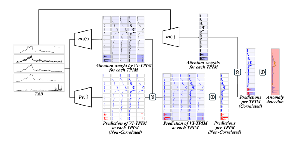 Figure 1: General architecture of TAIL-MIL (adapted from Jang & Kwon, AAAI 2025).
Conclusion
TAIL-MIL offers an elegant and principled solution for multivariate time series anomaly detection and localization under weak supervision:
- Targeted Context Modeling: T-Attention and V-Attention capture temporal patterns and inter-variable correlations to distribute attention weights appropriately.
- Bottom-Up Supervision: Sequence-level decisions are linear combinations of instance-level predictions, delivering native interpretability and multi-scale detection.
- Local Signal Preservation: Elementary scores are calculated on untampered local representations, preventing localized anomaly signals from being washed out by surrounding noise.
Reference
- J.~Jang and H.-Y.~Kwon, TAIL-MIL: Time-Aware and Instance-Learnable Multiple Instance Learning for Multivariate Time Series Anomaly Detection, Proceedings of the AAAI Conference on Artificial Intelligence, vol. 39, no. 17, pp. 17582–17589, 2025.
Weekly Notes
Every Sunday, I share what I've been learning: papers, ideas, experiments, and questions that stayed with me.
You can unsubscribe at any time with a single click.
Discussion about this post0
Join the discussion
A secure sign-in link will be sent to your email address.
Loading discussion...