

Introduction: The Data Preparation Pipeline
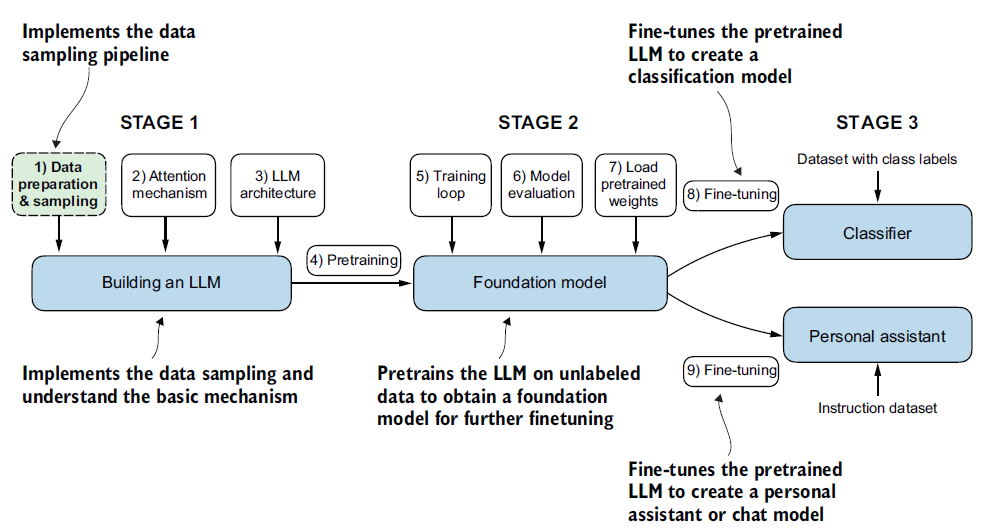
Before even thinking about the architecture or the training of an LLM, the most crucial step is preparing the training data. That is the purpose of the very first step of phase 1 in developing a language model.
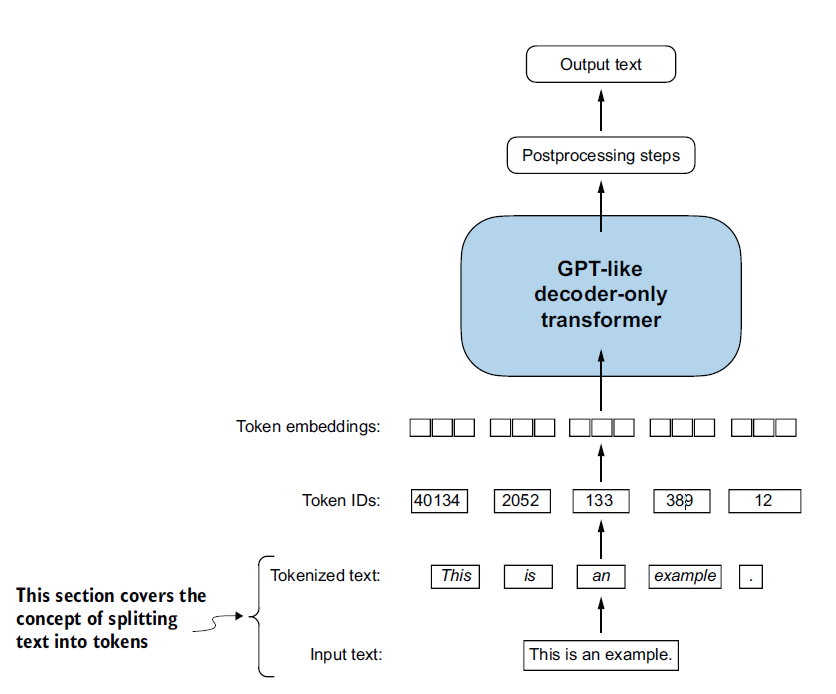
To process text, an LLM does not read raw sentences. It converts the text through a well-defined pipeline:
- Tokenization: The raw text is split into small units called tokens (which can be whole words or subwords). Advanced methods such as Byte Pair Encoding (BPE) are generally used in recent models like GPT.
- Sampling: With a “sliding window” approach, we extract input/output pairs used to train the model on the next-word prediction task.
- Vectorization: The extracted tokens are then converted into vectors of numbers (embeddings) that the neural network can ingest and process mathematically.
Understanding Word Embeddings
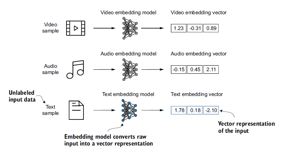
Neural networks cannot process raw text directly, because the algorithms need continuous numerical values to work. The method for achieving this is called embedding.
An embedding projects discrete objects (words, sentences, audio, images) to points in a format the machine can process: a continuous vector space (a sequence of numbers). It is important to understand that each data format has its own kind of embedding model (you cannot use a text model on video).
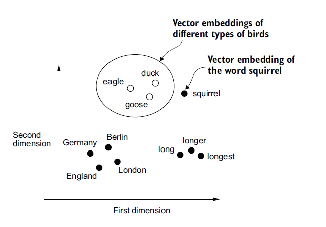
In this book, we focus only on word embeddings, since LLMs generate one word at a time. Historically, third-party models such as Word2Vec were used to turn each word into a vector. The mathematical logic is elegant: words that share similar contexts get similar values and therefore end up clustered together geometrically when plotted in a two-dimensional space.
Modern LLMs, however, do not rely on Word2Vec. They use their own built-in embedding layer, which is trained and optimized together with the rest of the model, so the vectors adapt to the exact characteristics of the target data.
Finally, the dimensionality of these vectors matters: a two-dimensional space is useful for teaching and visualization (as in figure 2.3), but in a real model the number of dimensions grows quickly to capture all the expressiveness and nuance of language. More dimensions mean more precision, at the cost of computational efficiency. A small GPT-2 uses 768 dimensions for a single word, while the huge GPT-3 needs 12,288!
Tokenizing Text
Tokenization is an essential preprocessing step before creating embeddings for an LLM. It consists of splitting the input text into individual tokens, which can be single words or special characters, including punctuation.
In this section, we use Edith Wharton’s short story “The Verdict”, which is in the public domain.
You can download and read the text with the following Python code:
import urllib.request
url = ("https://raw.githubusercontent.com/rasbt/"
       "LLMs-from-scratch/main/ch02/01_main-chapter-code/"
       "the-verdict.txt")
file_path = "the-verdict.txt"
urllib.request.urlretrieve(url, file_path)

with open("the-verdict.txt", "r", encoding="utf-8") as f:
    raw_text = f.read()

print("Total number of character:", len(raw_text))
print(raw_text[:99])
Output:
Total number of character: 20479
I HAD always thought Jack Gisburn rather a cheap genius--though a good fellow
enough--so it was no
Although training real LLMs often involves millions of articles (gigabytes of text), we use this 20,479-character sample for educational purposes, so the code runs in reasonable time on consumer hardware.
A simple tokenizer with regular expressions
To split the text into a list of tokens, we take a short detour through Python’s regular expression library (re).
We avoid converting the whole text to lowercase, because capitalization helps LLMs:
- Distinguish proper nouns from common nouns.
- Understand sentence structure.
- Learn to generate text with correct capitalization.
Here is a first attempt that splits on whitespace only:
import re
text = "Hello, world. This, is a test."
result = re.split(r'(\s)', text)
print(result)
Output:
['Hello,', ' ', 'world.', ' ', 'This,', ' ', 'is', ' ', 'a', ' ', 'test.']This scheme mostly works, but punctuation stays attached to the words ("Hello,"). To fix this, let’s also split on commas and periods (r'([,.]|\s)'):
result = re.split(r'([,.]|\s)', text)
print(result)
Output:
['Hello', ',', '', ' ', 'world', '.', '', ' ', 'This', ',', '', ' ', 'is', ' ', 'a', ' ', 'test', '.', '']One small problem remains: the list still contains whitespace and empty strings. We can remove these extra characters with .strip():
result = [item for item in result if item.strip()]
print(result)
Output:
['Hello', ',', 'world', '.', 'This', ',', 'is', 'a', 'test', '.']A note on whitespace: When building a simple tokenizer, whether you encode whitespace as separate characters or remove it (with
.strip()) depends on your application. Removing it reduces memory and compute requirements. Keeping it, however, is useful for models that are sensitive to the exact structure of the text (such as Python code, which is indentation-sensitive). Here, we remove it for simplicity.
Let’s extend the regular expression to handle other punctuation marks and double dashes, like the ones found in “The Verdict”:
text = "Hello, world. Is this-- a test?"
result = re.split(r'([,.:;?_!"()\']|--|\s)', text)
result = [item.strip() for item in result if item.strip()]
print(result)
Output:
['Hello', ',', 'world', '.', 'Is', 'this', '--', 'a', 'test', '?']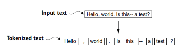
Now that we have a working basic tokenizer, let’s apply it to Edith Wharton’s entire short story:
preprocessed = re.split(r'([,.:;?_!"()\']|--|\s)', raw_text)
preprocessed = [item.strip() for item in preprocessed if item.strip()]

print(len(preprocessed))
print(preprocessed[:30])
Output:
4690
['I', 'HAD', 'always', 'thought', 'Jack', 'Gisburn', 'rather', 'a', 'cheap', 'genius', '--', 'though', 'a', 'good', 'fellow', 'enough', '--', 'so', 'it', 'was', 'no', 'great', 'surprise', 'to', 'me', 'to', 'hear', 'that', ',', 'in']
Converting Tokens into Token IDs
Once the text has been split into tokens (strings), the next step is to convert them into integers (token IDs). This is a mandatory intermediate step before generating the embedding vectors.
To turn tokens into IDs, we first need to build a vocabulary. This vocabulary maps each unique word and special character to a unique integer.
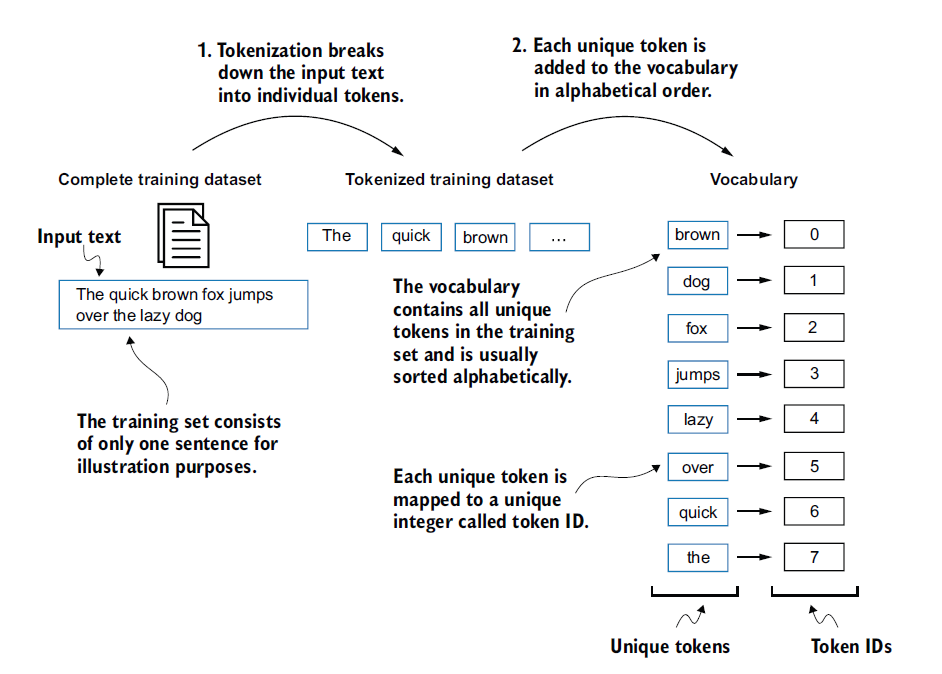
Let’s create the list of all unique tokens and sort them to determine the size of our vocabulary:
all_words = sorted(set(preprocessed))
vocab_size = len(all_words)
print(vocab_size)
Output:
1130The vocabulary contains 1,130 different tokens. We can now create the dictionary that maps each token to a number:
vocab = {token:integer for integer,token in enumerate(all_words)}
for i, item in enumerate(vocab.items()):
    print(item)
    if i >= 50:
        break
Output:
('!', 0)
('"', 1)
("'", 2)
...
('Her', 49)
('Hermia', 50)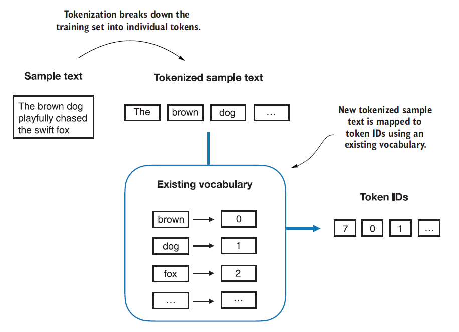
Implementing a Tokenizer class
To automate this process, we implement a Python class, SimpleTokenizerV1. It includes:
- An
encode()method that splits a text into tokens and turns them into IDs. - A
decode()method that performs the reverse operation (from token IDs back to text), which is essential for reading the output generated by the model.
class SimpleTokenizerV1:
    def __init__(self, vocab):
        self.str_to_int = vocab  # Stores the vocabulary for encoding
        self.int_to_str = {i:s for s,i in vocab.items()}  # Inverse vocabulary for decoding

    def encode(self, text):
        preprocessed = re.split(r'([,.?_!"()\']|--|\s)', text)
        preprocessed = [item.strip() for item in preprocessed if item.strip()]
        ids = [self.str_to_int[s] for s in preprocessed]
        return ids

    def decode(self, ids):
        text = " ".join([self.int_to_str[i] for i in ids])
        # Removes the spaces inserted before punctuation
        text = re.sub(r'\s+([,.?!"()\'])', r'\1', text)
        return text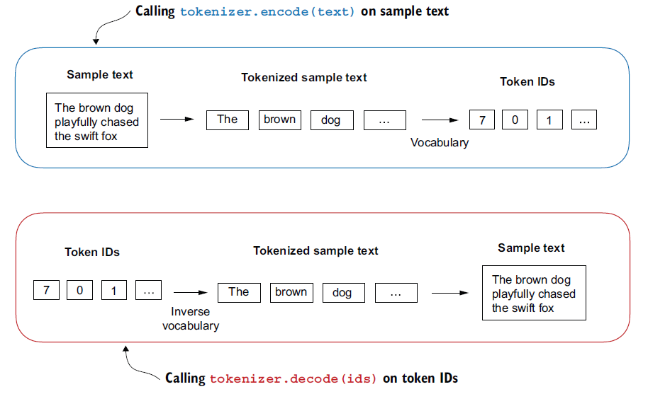
Let’s test our class on an excerpt from the story:
tokenizer = SimpleTokenizerV1(vocab)
text = """"It's the last he painted, you know,"
Mrs. Gisburn said with pardonable pride."""
ids = tokenizer.encode(text)
print(ids)
Output:
[1, 56, 2, 850, 988, 602, 533, 746, 5, 1126, 596, 5, 1, 67, 7, 38, 851, 1108, 754, 793, 7]Now let’s decode this list of IDs to check whether we get the original sentence back:
print(tokenizer.decode(ids))Output:
'" It\' s the last he painted, you know," Mrs. Gisburn said with pardonable pride.'The decoder works! Now let’s try a new text that does not come from Edith Wharton’s story:
text = "Hello, do you like tea?"
print(tokenizer.encode(text))
Output:
KeyError: 'Hello'Problem: The word “Hello” does not appear in “The Verdict”, so it is missing from our vocabulary. This shows why LLMs must be trained on huge, diverse datasets to broaden their vocabulary (and why we will need special tokens to handle unknown words).
Adding Special Context Tokens
We need to modify the tokenizer to handle unknown words. Adding special context tokens also improves the model’s understanding, for example by marking the start or the end of a document. We will add two new tokens: <|unk|> for unknown words, and <|endoftext|> to separate independent text documents.
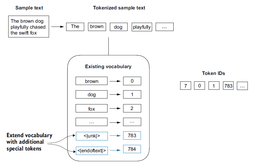
<|unk|> (for unknown words) and <|endoftext|> (to separate two unrelated text sources) to the vocabulary. Source: Raschka (2024).The <|endoftext|> token is crucial when training GPT-style LLMs on many independent documents or books. It helps the model understand that, although these texts are concatenated back to back for training, they have no contextual link to each other.
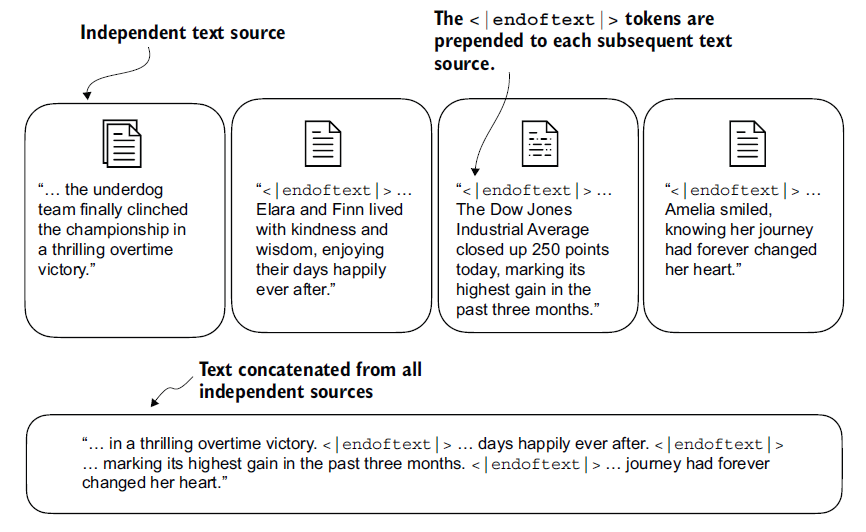
<|endoftext|> token acts as a marker signaling the start or the end of a segment. Source: Raschka (2024).Updating the Vocabulary
Let’s append these two special tokens to our list of unique words, then check the new vocabulary size:
all_tokens = sorted(list(set(preprocessed)))
all_tokens.extend(["<|endoftext|>", "<|unk|>"])
vocab = {token:integer for integer,token in enumerate(all_tokens)}
print(len(vocab.items()))
Output:
1132The vocabulary now contains 1,132 entries (instead of 1,130). Let’s print the last five entries of the dictionary to confirm:
for i, item in enumerate(list(vocab.items())[-5:]):
    print(item)
Output:
('younger', 1127)
('your', 1128)
('yourself', 1129)
('<|endoftext|>', 1130)
('<|unk|>', 1131)
Tokenizer V2: Handling Unknown Words
We can adjust the encode method of our previous class. From now on, if a word in the input text is not in our self.str_to_int lookup, it is automatically mapped to the <|unk|> token.
class SimpleTokenizerV2:
    def __init__(self, vocab):
        self.str_to_int = vocab
        self.int_to_str = { i:s for s,i in vocab.items()}

    def encode(self, text):
        preprocessed = re.split(r'([,.:;?_!"()\']|--|\s)', text)
        preprocessed = [item.strip() for item in preprocessed if item.strip()]

        # Safety filter for unknown words
        preprocessed = [item if item in self.str_to_int else "<|unk|>" for item in preprocessed]
        ids = [self.str_to_int[s] for s in preprocessed]
        return ids

    def decode(self, ids):
        text = " ".join([self.int_to_str[i] for i in ids])
        text = re.sub(r'\s+([,.:;?!"()\'])', r'\1', text)
        return text
Let’s test this new version on a sample made of two independent sentences joined with our marker. First, the test text:
text1 = "Hello, do you like tea?"
text2 = "In the sunlit terraces of the palace."
text = " <|endoftext|> ".join((text1, text2))
print(text)
Output:
Hello, do you like tea? <|endoftext|> In the sunlit terraces of the palace.Now let’s encode the full text and look at the generated IDs:
tokenizer = SimpleTokenizerV2(vocab)
print(tokenizer.encode(text))
Output:
[1131, 5, 355, 1126, 628, 975, 10, 1130, 55, 988, 956, 984, 722, 988, 1131, 7](We can see token 1130, which corresponds to <|endoftext|>, and two occurrences of 1131 for <|unk|>, corresponding to the out-of-vocabulary words.)
Let’s decode the IDs to see it for ourselves:
print(tokenizer.decode(tokenizer.encode(text)))Output:
<|unk|>, do you like tea? <|endoftext|> In the sunlit terraces of the <|unk|>.Comparing this detokenized text with the original input, we can tell that the training dataset, Edith Wharton’s short story “The Verdict”, does not contain the words “Hello” and “palace”. These words have therefore been replaced with <|unk|>.
Other Kinds of Context Tokens
Depending on the LLM, some researchers also use additional special tokens such as:
[BOS](Beginning of sequence): This token marks the start of a text. It tells the LLM where a piece of content begins.[EOS](End of sequence): This token is placed at the end of a text and is especially useful when concatenating several unrelated texts, much like<|endoftext|>. For example, when combining two different Wikipedia articles or books, the[EOS]token indicates where one ends and the next one begins.[PAD](Padding): When training LLMs with batch sizes larger than one, a batch can contain texts of different lengths. To make sure all texts have the same length, the shorter ones are extended, or “padded”, with the[PAD]token until they reach the length of the longest text in the batch.
What makes the GPT tokenizer special
The tokenizer used by GPT models stands out for its simplicity. Instead of multiplying special tokens, it only uses
<|endoftext|>, as the equivalent of both[BOS]and[EOS].This
<|endoftext|>token is also used for padding. When training in batches, a mask is applied so that the model simply ignores these padding tokens. The specific token chosen for padding therefore does not matter.Finally, this tokenizer does not use an
<|unk|>token for out-of-vocabulary words. Instead, it uses an algorithm called Byte Pair Encoding (BPE), which breaks unknown words down into subword units, as we will see in the next section.
Byte Pair Encoding (BPE)
Let’s look at a more sophisticated tokenization scheme based on a concept called Byte Pair Encoding (BPE). The BPE tokenizer was used to train LLMs such as GPT-2, GPT-3 and the original model used in ChatGPT.
Here, we use an existing open-source Python library called tiktoken (https://github.com/openai/tiktoken), which implements the BPE algorithm very efficiently. As with other Python libraries, we can install tiktoken with the pip package installer from the terminal:
pip install tiktokenChecking the version:
from importlib.metadata import version
import tiktoken

print("tiktoken version:", version("tiktoken"))
Output:
tiktoken version: 0.7.0Initializing a BPE tokenizer (the “gpt2” model):
tokenizer = tiktoken.get_encoding("gpt2")Encoding a text (including the context control tokens):
text = (
    "Hello, do you like tea? <|endoftext|> In the sunlit terraces"
    "of someunknownPlace."
)
# allowed_special keeps the tokenizer from raising an error when it sees <|endoftext|>
integers = tokenizer.encode(text, allowed_special={"<|endoftext|>"})
print(integers)
Output:
[15496, 11, 466, 345, 588, 8887, 30, 220, 50256, 554, 262, 4252, 18250, 8812, 2114, 286, 617, 34680, 27271, 13]Decoding back:
strings = tokenizer.decode(integers)
print(strings)
Output:
Hello, do you like tea? <|endoftext|> In the sunlit terraces of someunknownPlace.Key Observations on the BPE Tokenizer
This experiment highlights two remarkable facts about the BPE tokenizer of the GPT family:
- The position of the
<|endoftext|>token: Its assigned ID is very large (50256). This makes sense: the total vocabulary of GPT-2 or GPT-3 style models is limited to 50,257 tokens, with<|endoftext|>in the very last position. - Robust handling of out-of-vocabulary (OOV) words: The tokenizer encodes and decodes
someunknownPlaceperfectly, without having to fall back to a blind token like<|unk|>.
How does BPE do without the <|unk|> token entirely?
The strength of BPE lies in its ability to split a completely unknown word. Instead of raising an error or bluntly replacing it with <|unk|>, BPE breaks the word into smaller known fragments: syllables or subwords, or, as a last resort, individual characters or bytes.
Figure 2.11: BPE tokenizers break unknown words down into subwords and individual characters. This way, a BPE tokenizer can parse any word and never needs to replace unknown words with special tokens such as
<|unk|>. Source: Raschka (2024).
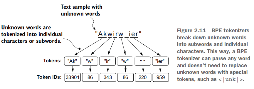
This ability to break unknown words down into individual characters guarantees that the tokenizer, and therefore the LLM, can process any text, even if it contains words absent from its training data.
Exercise 2.1: Byte Pair Encoding of Unknown Words
Try the BPE tokenizer from the
tiktokenlibrary on the unknown word “Akwirw ier” and print the individual token IDs. Then call the decode function on each of the integers in that list to reproduce the mapping produced by BPE. Finally, call the decode method on the full list of token IDs to check whether it rebuilds the original input from figure 2.11.
Solution:
Passing each subfragment of the word from figure 2.11 to the tokenizer by hand:
print(tokenizer.encode("Ak"))
print(tokenizer.encode("w"))
# ...
Output:
[33901]
[86]
# ...
Once assembled, a single call passes the list of IDs back to the tokenizer, which faithfully rebuilds the original string:
print(tokenizer.decode([33901, 86, 343, 86, 220, 959]))Output:
Akwirw ierIn short, BPE builds its vocabulary gradually, starting from the smallest unit. It first initializes its vocabulary with all the individual characters (“a”, “b”, and so on). It then finds the characters that most often appear side by side and merges them into subwords. For example, if “d” and “e” are very often adjacent, they are merged into the subword “de” (very common in words like “define” or “made”). This process repeats iteratively, merging the most frequent subwords into whole words, based purely on how often they occur.
Data Sampling with a Sliding Window
To train an LLM, we generate input-target pairs. Since the model’s task is to predict the next word, the target sequence (y) is exactly the input sequence (x) shifted one position to the right.
Figure 2.12: Extracting input blocks from a text sample to train the LLM. The task is to predict the word that follows the input block, masking the words that come after the target. (Tokenization is omitted here for clarity.). Source: Raschka (2024).
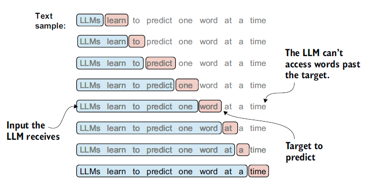
To create these pairs, we slide a window over the tokenized text. The context size (context_size or max_length) determines how many tokens the input contains.
# Shifting by one position to create the target
context_size = 4
x = enc_sample[:context_size]
y = enc_sample[1:context_size+1]
print(f"x: {x}") # [290, 4920, 2241, 287]
print(f"y: {y}") # [4920, 2241, 287, 257]
Implementing the Data Pipeline with PyTorch
For training, the data must be converted into tensors and organized into batches. We use two standard PyTorch classes for this: Dataset and DataLoader.
Figure 2.13: For maximum efficiency, the inputs are gathered into a tensor
x, where each row is an input context. A second tensoryholds the corresponding prediction targets (the next words), created by shifting the input by one position. Source: Raschka (2024).
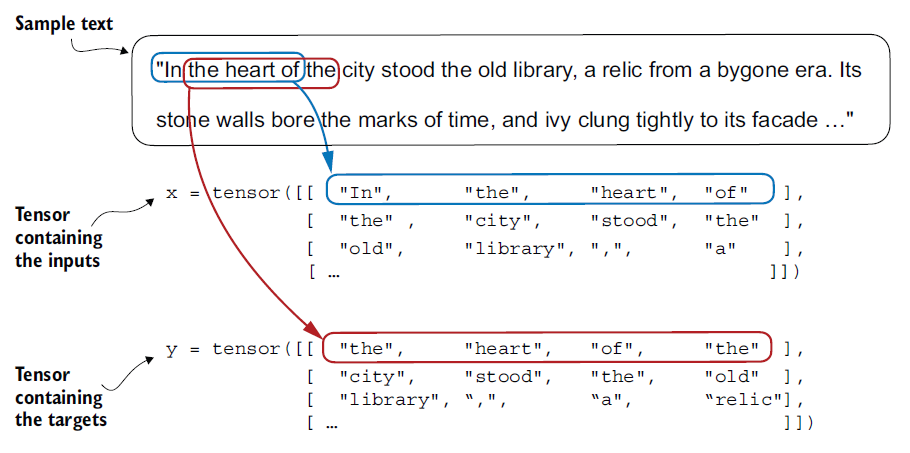
1. The Dataset class (GPTDatasetV1):
This class defines how the text is cut into individual sequences. It splits the text into chunks of max_length tokens for the inputs, and creates the matching target chunks by shifting them by one token.
import torch
from torch.utils.data import Dataset, DataLoader

class GPTDatasetV1(Dataset):
    def __init__(self, txt, tokenizer, max_length, stride):
        self.input_ids = []
        self.target_ids = []

        # Tokenize the whole text
        token_ids = tokenizer.encode(txt)

        # Use a sliding window to create the sequences
        for i in range(0, len(token_ids) - max_length, stride):
            input_chunk = token_ids[i:i + max_length]
            target_chunk = token_ids[i + 1: i + max_length + 1]

            self.input_ids.append(torch.tensor(input_chunk))
            self.target_ids.append(torch.tensor(target_chunk))

    def __len__(self):
        return len(self.input_ids)

    def __getitem__(self, idx):
        return self.input_ids[idx], self.target_ids[idx]
2. The DataLoader class:
The DataLoader groups the sequences from the Dataset into batches. This lets the model process several examples in parallel.
import tiktoken

def create_dataloader_v1(txt, batch_size=4, max_length=256, stride=128, shuffle=True, drop_last=True, num_workers=0):
    tokenizer = tiktoken.get_encoding("gpt2")
    dataset = GPTDatasetV1(txt, tokenizer, max_length, stride)

    dataloader = DataLoader(
        dataset,
        batch_size=batch_size,
        shuffle=shuffle,
        drop_last=drop_last,
        num_workers=num_workers
    )
    return dataloader
Important DataLoader Parameters
- Batch size: The number of sequences processed at once. A size of 1 is handy for illustration, but in deep learning we use larger batches to stabilize the model’s updates.
- Drop last (
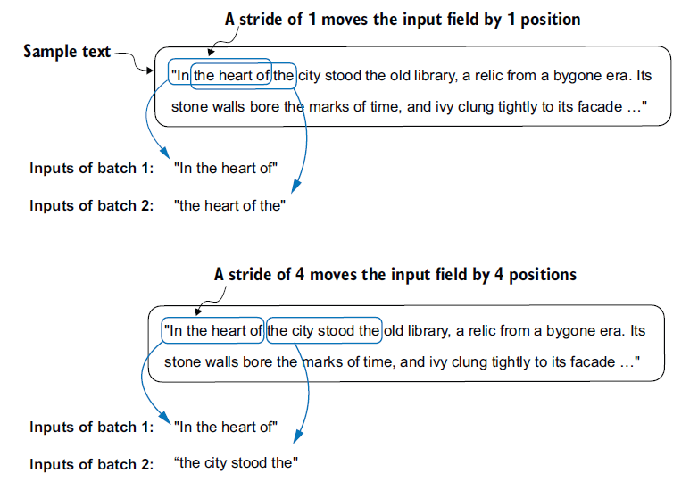
drop_last=True): If the total number of sequences is not divisible by the batch size, the last batch will be incomplete. Dropping it avoids instabilities (loss spikes) during training. - Stride: Determines how many positions the sliding window moves forward to extract the next sequence.
- A
strideof 1 moves the window by a single token, creating a lot of overlap between consecutive sequences (useful to visualize the mechanism). - In practice, during training,
strideis often set to the same value asmax_length. This prevents sequences from overlapping, which limits overfitting.
- A
Figure 2.14: Setting the stride equal to the input window size avoids any overlap between batches. Source: Raschka (2024).
Exercise 2.2: Data Loaders with Different Strides and Context Sizes
Try the data loader with other settings, such as
max_length=2andstride=2, ormax_length=8andstride=2, to build your intuition for how the sliding window works.
Creating Token Embeddings
The last step of data preparation is converting the token IDs into continuous embedding vectors. This vector representation is required because LLMs are deep neural networks trained with the backpropagation algorithm.
The weights of the embedding matrix are initialized with small random values that are optimized while the model trains.
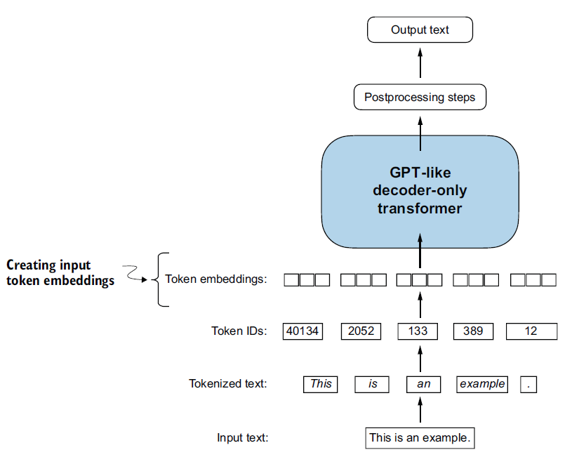
Figure 2.15: Preparing text involves tokenization, conversion into token IDs, and finally projecting these IDs into continuous vectors through an embedding layer. Source: Raschka (2024).
How an embedding layer works
We create such a layer with torch.nn.Embedding. Its dimensions depend on two parameters:
vocab_size: The size of the vocabulary (the number of rows).output_dim: The number of dimensions of each embedding vector (the number of columns).
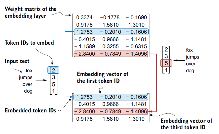
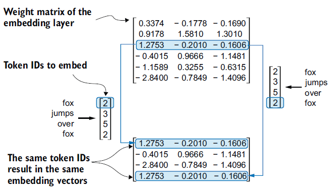
Passing a token ID to this layer performs a lookup operation: it directly retrieves the row of the matrix that corresponds to that ID.
# Retrieving vectors for input_ids = [2, 3, 5, 1]
# vocab_size = 6, output_dim = 3
print(embedding_layer(input_ids))

tensor([[ 1.2753, -0.2010, -0.1606],   # Row at index 2
        [-0.4015,  0.9666, -1.1481],   # Row at index 3
        [-2.8400, -0.7849, -1.4096],   # Row at index 5
        [ 0.9178,  1.5810,  1.3010]],  # Row at index 1
       grad_fn=<EmbeddingBackward0>)
Figure 2.16: Retrieving embedding vectors. Each token ID is used as an index to pull the matching row from the embedding layer’s weight matrix. Source: Raschka (2024).
A note on one-hot encoding: Using an embedding layer is mathematically equivalent to applying one-hot encoding followed by a matrix multiplication (a fully connected layer). The embedding layer, however, is a far more computationally efficient implementation, while remaining a differentiable component for backpropagation.
Encoding Word Positions
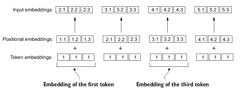
Token embeddings have a major structural flaw: whether a word appears at the start, in the middle or at the end of a sentence, its embedding vector is exactly the same. Worse, the self-attention mechanism of LLMs (covered in chapter 3) is, by construction, order-invariant: it treats the input sequence as a simple unordered set of tokens, with no notion of precedence or proximity.
token_id 5 always produces the same
embedding vector, whether it is in the first or the fourth position of the input
vector. Source: Raschka (2024).So we must inject position information into these embeddings for the network to understand word order.
There are two main families of positional encodings:
- Absolute positional encodings: A distinct position vector is associated with each index of the sequence (the token at position 0 gets one fixed vector, the one at position 1 another, and so on). These vectors have the same dimension as the token embeddings and are added to them element-wise. This is the approach OpenAI chose for its GPT models: the absolute position vectors are parameters learned and optimized during training, just like the network’s weights.
⚠️ Limit at inference time: The
pos_embedding_layeris a weight matrix of shape(context_length, output_dim). Withcontext_length = 1024, this matrix has exactly 1,024 rows, one per position, from index 0 to index 1,023. If, at inference time, we feed in a sequence of 1,500 tokens, the model tries to access rows 1,024 to 1,499, which do not exist. PyTorch immediately raises an error:IndexError: index out of range in self. The model does not degrade gracefully: it crashes. That is why any sequence longer thancontext_lengthmust be truncated before being passed to the model.
- Relative positional encodings: Rather than encoding the absolute position of each token, this kind of encoding models the distance between two tokens, that is, how far apart they are in the sequence. Concretely, instead of injecting a position vector into the input embedding, the positional information is built directly into the attention score computation between two tokens and : the score then depends on rather than on and separately.
The main benefit is better out-of-distribution generalization: the model has never memorized a fixed vector per absolute position; it has learned to reason in terms of gaps between tokens, which stay valid whatever the total length of the sequence.
Implementation in PyTorch
In the GPT approach (absolute positions), we create two separate torch.nn.Embedding layers, both with the same output dimension:
- One layer to encode the meaning of the tokens (indexed over the vocabulary).
- One layer to encode the position of the tokens in the sequence.
Here we work with an embedding dimension of 256 (smaller than GPT-3’s 12,288 dimensions, but enough for experimentation) and the BPE tokenizer introduced earlier, which covers a vocabulary of 50,257 tokens.
Step 1. Create the token embedding layer
vocab_size = 50257
output_dim = 256

token_embedding_layer = torch.nn.Embedding(vocab_size, output_dim)
Step 2. Load a batch from the DataLoader
First, let’s create the DataLoader (see section 2.6) to fetch a batch of examples:
max_length = 4
dataloader = create_dataloader_v1(
    raw_text, batch_size=8, max_length=max_length,
    stride=max_length, shuffle=False
)
data_iter = iter(dataloader)
inputs, targets = next(data_iter)

print("Token IDs:\n", inputs)
print("\nInputs shape:\n", inputs.shape)
Token IDs:
tensor([[ 40, 367, 2885, 1464],
[1807, 3619, 402, 271],
[10899, 2138, 257, 7026],
[15632, 438, 2016, 257],
[ 922, 5891, 1576, 438],
[ 568, 340, 373, 645],
[ 1049, 5975, 284, 502],
[ 284, 3285, 326, 11]])
Inputs shape:
torch.Size([8, 4])The inputs tensor has shape (8, 4): 8 text examples, each made of 4 tokens.
Step 3. Apply the token embedding
token_embeddings = token_embedding_layer(inputs)
print(token_embeddings.shape)
torch.Size([8, 4, 256])Each token_id is now represented by a 256-dimensional vector.
Step 4. Create the positional embedding layer
context_length = max_length  # Maximum length of the input sequence

pos_embedding_layer = torch.nn.Embedding(context_length, output_dim)
pos_embeddings = pos_embedding_layer(torch.arange(context_length))
print(pos_embeddings.shape)
torch.Size([4, 256])
torch.arange(context_length)simply generates[0, 1, 2, ..., context_length - 1].
This is the list of every position index, passed to the layer to fetch all the rows at once: the vector for position 0, then the one for position 1, and so on.
Step 5. Add them up to form the final input
input_embeddings = token_embeddings + pos_embeddings
print(input_embeddings.shape)
torch.Size([8, 4, 256])Thanks to PyTorch’s broadcasting mechanism, the pos_embeddings tensor of shape (4, 256), identical for every example in the batch, is automatically added to each of the 8 examples in token_embeddings, of shape (8, 4, 256). This final input_embeddings tensor is what gets passed to the model’s deeper layers.
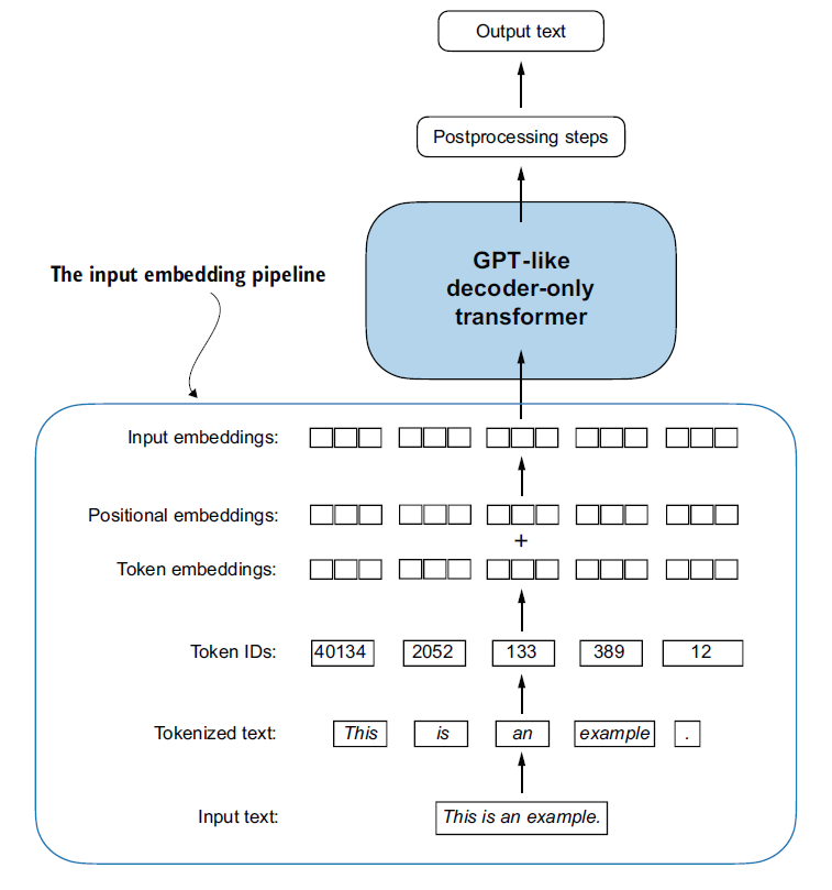
token_ids and turned into token embeddings, to which the positional embeddings are added to form the input_embeddings passed to the main layers of the LLM. Source: Raschka (2024).Summary
-
LLMs do not process raw text: The text must first be split into tokens (words or subwords), then turned into integers called
token_ids. -
Special tokens: Markers such as
<|unk|>or<|endoftext|>are used to structure the data and to separate independent texts during training. -
The BPE (Byte Pair Encoding) tokenizer: It lets LLMs like GPT-2 or GPT-3 handle any unknown word by breaking it down into subwords or characters.
-
Sliding window sampling: During training, the targets (labels) are extracted with a simple +1 shift, teaching the model to always predict the next token.
-
The
Embeddinglayer in PyTorch: It behaves like a lookup table: given an integertoken_id, it instantly returns the matching vector. Mathematically, this is equivalent to encoding the token as a one-hot vector and multiplying it by a linear projection matrix, but the direct implementation is drastically more efficient. -
Semantic embedding: Turning an abstract token into a continuous vector places words in a high-dimensional vector space, where semantic relationships can be optimized numerically.
-
Positional encoding: The
self-attentionmechanism reads a sequence as an unordered set of tokens. To give it back a sense of order, GPT adds a learned absolute position vector to each token embedding (one vector per sequence index), stored in a matrix of shape(context_length, output_dim). This matrix imposes a hard constraint: any sequence longer thancontext_lengthtokens must be truncated, or an index error will occur at inference time. More recent architectures prefer relative encodings, built into the attention score computation rather than added to the embeddings, which removes this length limit.
Weekly Notes
Every Sunday, I share what I've been learning: papers, ideas, experiments, and questions that stayed with me.
You can unsubscribe at any time with a single click.
Discussion about this post0
Join the discussion
A secure sign-in link will be sent to your email address.
Loading discussion...