Introduction to PyTorch

Introduction

Welcome to Chapter 0 of our series on building an LLM (Large Language Model) from scratch. Before diving into attention mechanisms and the Transformer architecture, we need to master our main tool: PyTorch.

PyTorch is an extremely popular deep learning library, valued for its flexibility and its intuitive handling of tensors. In this preliminary chapter, we explore the fundamental concepts that will serve as the foundation for the rest of the project:

• Creating and manipulating tensors (the data structures at the heart of neural networks).
• How computation graphs work.
• The magic of autograd (the automatic differentiation engine that lets models learn through gradient descent).

If you are already comfortable with PyTorch, you can skim this chapter or go straight to Chapter 1. Otherwise, open your Python environment (or Google Colab), and let’s get started!

import torch
torch.__version__

'2.10.0+cu128'

import torch
torch.cuda.is_available()

True

Understanding Tensors

Creating tensors and choosing their type

tensor0d = torch.tensor(1)

tensor1d = torch.tensor([1, 2, 3])

tensor2d = torch.tensor([[1, 2, 3], 
                         [4, 5, 6]])

tensor3d = torch.tensor([[[1, 2], [3, 4]], 
                         [[5, 6], [8, 9]]])

print(tensor1d.dtype)

torch.int64

float_tensor = torch.tensor([1.0, 2.0, 3.0])
print(float_tensor.dtype)

torch.float32

32-bit floating-point numbers offer enough precision for most deep learning tasks while using less memory and compute than 64-bit floating-point numbers. What’s more, GPU architectures are optimized for 32-bit computation, and using this data type can considerably speed up model training and inference. The precision can also be changed with a tensor’s ‘.to’ method.

float_tensor = float_tensor.to(torch.float32)
print(float_tensor.dtype)

torch.float32

print(tensor2d)

tensor([[1, 2, 3],
        [4, 5, 6]])

Shape and reshaping: .reshape() and .view()

The .shape attribute gives us access to a tensor’s shape:

print(tensor2d.shape)

torch.Size([2, 3])

To reshape the tensor into a 3 × 2 tensor, we can use the .reshape method:

print(tensor2d.reshape([3, 2]))

tensor([[1, 2],
        [3, 4],
        [5, 6]])

Note, however, that the most common command for reshaping tensors in PyTorch is .view()

print(tensor2d.view([3, 2]))

tensor([[1, 2],
        [3, 4],
        [5, 6]])

The subtle difference between .view() and .reshape() in PyTorch lies in how they handle memory layout: .view() requires the original data to be contiguous and fails if it is not, while .reshape() works in every case, copying the data if necessary to produce the requested shape.

Forget the math for a moment and picture how your computer’s physical memory (RAM or VRAM) works.

What is “physical data”?

Your computer’s memory has no concept of a “2D array” or a “3D cube”. Memory is simply a very long straight line of small boxes.

Say you create a simple PyTorch tensor, an array with 2 rows and 2 columns:

t = torch.tensor([[1, 2],
                  [3, 4]])

Visually (logically), you see a square. Physically (in RAM), PyTorch stores these numbers in 4 boxes lined up one after the other: [1, 2, 3, 4].

When PyTorch wants to read the first row [1, 2], it reads the first two boxes. For the second row [3, 4], it reads the next two. Since the logical reading order matches the order of the physical boxes exactly, we say the tensor is contiguous (neatly stored).

How a tensor becomes non-contiguous

Now let’s apply a mathematical operation, for example transposition (which swaps rows and columns).

t_transpose = t.t()
# Logical result (what you see on screen):
# [[1, 3],
#  [2, 4]]

Here is PyTorch’s secret to being ultra-fast: it does not move anything in the physical boxes! In RAM, the boxes are still in the order [1, 2, 3, 4].

To show you [[1, 3], [2, 4]], PyTorch just added an internal note that says: “Careful: to read the first row, take box no. 1, then jump over no. 2 to fetch box no. 3.”

Since PyTorch now has to “jump” from box to box to read the array correctly, the reading order no longer matches the physical order of the boxes. The tensor has become non-contiguous. That is what a “complex modification” means: an operation that changes the logical shape without touching the physical layout. (Cutting out part of the tensor with slicing, such as t[:, 1], does exactly the same thing.)

Why .view() fails

The .view() function gives a tensor a new shape (for example, turning our 2x2 into a row of 4). But .view() has a technical limitation: it refuses to work if it has to skip boxes. It wants to read the boxes neatly from left to right.

If you run t_transpose.view(4), PyTorch panics: “Hey, this tensor asks me to jump around in physical memory, I can’t do a .view() on it!” -> Error (crash).

Why .reshape() always works

The .reshape(4) function is much smarter. When you run it on t_transpose:

1. It looks at physical memory and realizes: “Ah, there are jumps, it’s non-contiguous.”
2. Instead of crashing, it quietly builds new physical boxes somewhere else in RAM and stores them in the right, direct order: [1, 3, 2, 4].
3. Now that everything is tidy, it applies the new shape. -> Success, no crash.

That is why .reshape() is said to “copy the data if necessary”, and why it is the recommended method if you want peace of mind!

Transposing and multiplying matrices

We can use .T to transpose a tensor, which means flipping it over its diagonal

print(tensor2d.T)

tensor([[1, 4],
        [2, 5],
        [3, 6]])

The usual way to multiply two matrices in PyTorch is the .matmul method

print(tensor2d.matmul(tensor2d.T))

tensor([[14, 32],
        [32, 77]])

Seeing Models as Computation Graphs

PyTorch’s autograd system provides functions to automatically compute gradients in dynamic computation graphs. A computation graph is a directed graph that lets us express and visualize mathematical expressions. In the context of deep learning, a computation graph lays out the sequence of calculations needed to compute the output of a neural network. We will need it to compute the gradients required for backpropagation, the main training algorithm for neural networks.

The forward pass of a logistic regression

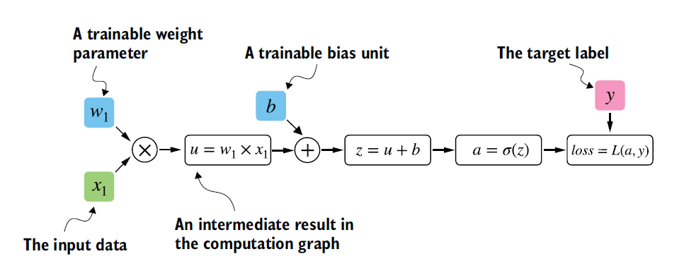
The forward pass of a logistic regression represented as a computation graph. The input feature x1 is multiplied by a model weight w1 and passed through an activation function σ after the bias is added. The loss is computed by comparing the model output a with a given label y. Source: Raschka (2024).

# This import statement is a common PyTorch convention to avoid long lines of code
import torch.nn.functional as F

# True label
y = torch.tensor([1.0])

# Input feature
x1 = torch.tensor([1.1])

# Weight parameter
w1 = torch.tensor([2.2])

# Bias unit
b = torch.tensor([0.0])

# Net input
z1 = x1 * w1 + b

# Activation and output 
a = torch.sigmoid(z1)

loss = F.binary_cross_entropy(a, y)

Automatic Differentiation Made Easy

When we run computations in PyTorch, it builds a computation graph internally by default if one of its leaf nodes has its requires_grad attribute set to True. This is useful when we want to compute gradients. Gradients are essential for training neural networks with the well-known backpropagation algorithm, which can be seen as an application of the chain rule from calculus to neural networks, as shown in the figure below:

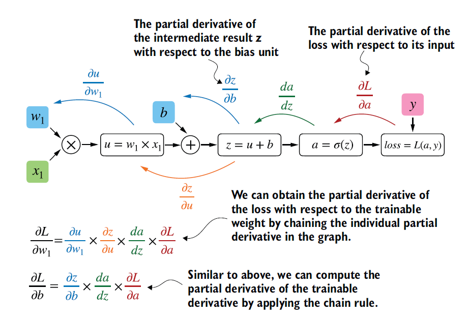
The most common way to compute the gradients of the loss in a computation graph is to apply the chain rule from right to left, also called reverse-mode automatic differentiation or backpropagation. We start from the output layer (or the loss itself) and work backward through the network to the input layer. We do this to compute the gradient of the loss with respect to each parameter (weights and biases) of the network, which tells us how to update these parameters during training. Source: Raschka (2024).

• Partial derivatives measure how fast a function changes with respect to one of its variables.

• A gradient is a vector containing all the partial derivatives of a multivariate function (a function with more than one input variable).

Put simply, all you need to know is that the chain rule is a way to compute the gradients of a loss function with respect to the model parameters in a computation graph. This provides the information needed to update each parameter so as to minimize the loss function (which serves as a proxy for measuring the model's performance, using a method such as gradient descent).

Computing gradients with grad

PyTorch’s autograd engine builds a computation graph in the background by tracking every operation performed on tensors. Then, by calling the grad function, we can compute the gradient of the loss with respect to the model parameter w1, as shown in the following listing.

import torch.nn.functional as F
from torch.autograd import grad

y = torch.tensor([1.0])
x1 = torch.tensor([1.1])
w1 = torch.tensor([2.2], requires_grad=True)
b = torch.tensor([0.0], requires_grad=True)

z1 = x1 * w1 + b
a = torch.sigmoid(z1)

loss = F.binary_cross_entropy(a, y)

By default, PyTorch destroys the computation graph after computing the gradients to free up memory. However, since we will reuse this computation graph shortly, we set retain_graph=True so that it stays in memory.

grad_L_w1 = grad(loss, w1, retain_graph=True)
grad_L_b = grad(loss, b, retain_graph=True)

print(grad_L_w1)
print(grad_L_b)

(tensor([-0.0898]),)
(tensor([-0.0817]),)

Here, we used the grad function manually, which can be useful for experimenting, debugging and demonstrating concepts.

Automating it with .backward()

But in practice, PyTorch provides higher-level tools to automate this process. For example, we can call .backward on the loss, and PyTorch will compute the gradients of all the leaf nodes in the graph, which are stored in the tensors’ .grad attributes.

loss.backward()
print(w1.grad)
print(b.grad)

tensor([-0.0898])
tensor([-0.0817])

Implementing a Multilayer Neural Network

Let’s look at a multilayer perceptron, a fully connected neural network, as shown in the figure below:

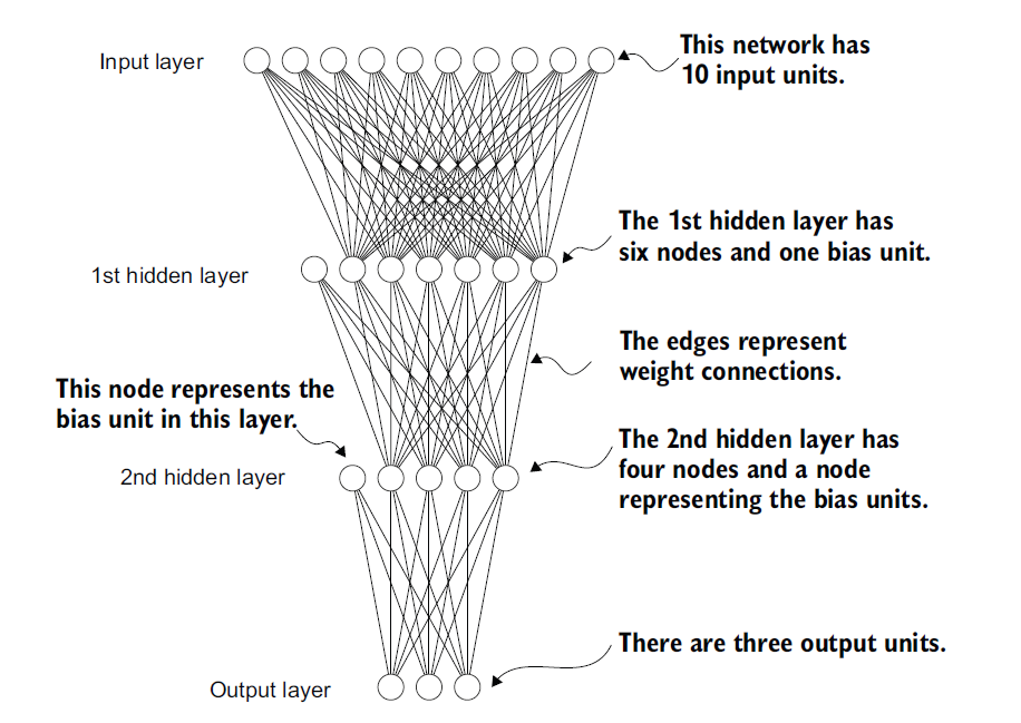
A multilayer perceptron with two hidden layers. Each node represents a unit in its layer. For illustration purposes, each layer has a very small number of nodes. Source: Raschka (2024).

Defining the architecture

When implementing a neural network in PyTorch, we can subclass torch.nn.Module to define our own custom network architecture. This Module base class provides a lot of functionality that makes building and training models easier. For example, it lets us encapsulate layers and operations and keep track of the model’s parameters.

Within this subclass, we define the network layers in the __init__ constructor and specify how the layers interact in the forward method.

The forward method describes how the input data flows through the network and comes together as a computation graph. The backward method, on the other hand, which we usually don’t need to implement ourselves, is used during training to compute the gradients of the loss function with respect to the model parameters.

class NeuralNetwork(torch.nn.Module):
    """Coding the number of inputs and oututs as variables allows us to reuse the same code for datasets with different numbers of features and classes."""

    def __init__(self, num_inputs, num_outputs):
        super().__init__()

        self.layers = torch.nn.Sequential(
            # 1st hidden layer 
            torch.nn.Linear(num_inputs, 30), # The Linear layer takes the number of input and output nodes as arguments
            torch.nn.ReLU(), # Nonlinear activation functions are placed between the hidden layers

            # 2nd hidden layer
            torch.nn.Linear(30, 20), # The number of output nodes of one hidden layer has to match the number of inputs of the next layer
            torch.nn.ReLU(),

            # output layer
            torch.nn.Linear(20, num_outputs), 
        )

    def forward(self, x):
        logits = self.layers(x)
        return logits # The outputs of the last layers are called logits

torch.nn.Sequential is not mandatory. It is simply a very handy shortcut (a “box”) for grouping layers that run one after another in a straight line.

The classic alternative, which is actually the most common approach, is to define each layer individually and then connect the pipes yourself in the forward() function.

class NeuralNetwork(torch.nn.Module):

    def __init__(self, num_inputs, num_outputs):
        super().__init__()

        # We define all our layers as separate attributes
        self.layer1 = torch.nn.Linear(num_inputs, 30)
        self.relu1 = torch.nn.ReLU()
        
        self.layer2 = torch.nn.Linear(30, 20)
        self.relu2 = torch.nn.ReLU()
        
        self.output_layer = torch.nn.Linear(20, num_outputs)

    def forward(self, x):
        # We manually pass the data 'x' from one layer to the next
        x = self.layer1(x)
        x = self.relu1(x)
        
        x = self.layer2(x)
        x = self.relu2(x)
        
        logits = self.output_layer(x)
        
        return logits

# We can now create an instance of our NeuralNetwork class and print it to see its architecture.
model = NeuralNetwork(50, 30)
print(model)

NeuralNetwork(
  (layer1): Linear(in_features=50, out_features=30, bias=True)
  (relu1): ReLU()
  (layer2): Linear(in_features=30, out_features=20, bias=True)
  (relu2): ReLU()
  (output_layer): Linear(in_features=20, out_features=30, bias=True)
)

Counting the trainable parameters

1. model.parameters()

This method comes from inheriting from torch.nn.Module. When we call model.parameters(), PyTorch walks through all the layers of our network on its own (our nn.Linear layers, whether or not they are inside a Sequential).

For each Linear layer, it “collects” two essential things:

1. The weight matrix (which connects the input to the output).
2. The bias vector (Activation functions such as ReLU have no weights or parameters, so they are simply skipped!)

It returns a list (a generator, to be precise) containing each of these big mathematical arrays (the tensors).

2. for p in ...

The loop goes through this list. On each iteration, p is a tensor (a weight matrix or a bias vector).

3. p.numel()

As we have seen, it counts the total number of values inside the tensor p. For example:

• If p is the weight matrix of the 1st layer (Linear(50, 30)), it counts $50 \times 30 = 1500$ elements.
• If p is the bias of that 1st layer, it counts $30$ elements.
• Total for this layer: 1530 parameters.

4. if p.requires_grad (the crucial detail)

This is a very clever filter. It tells the loop: “Only count the parameters that the optimizer is allowed to modify during training (requires_grad=True)”.

# To calculate the total number of trainable parameters in the model, we can use the following code:
num_params = sum(p.numel() for p in model.parameters() if p.requires_grad)
print("Total number of trainable model parameters:", num_params)

Total number of trainable model parameters: 2780

# We can access the corresponding weight parameter matrix as dollows :
print(model.layer1.weight)

Parameter containing:
tensor([[ 0.0220,  0.0694,  0.0166,  ..., -0.0385,  0.0019, -0.1359],
        [-0.0732,  0.0306, -0.0902,  ..., -0.0025,  0.0096,  0.0459],
        [ 0.0650,  0.0479, -0.0650,  ...,  0.0457,  0.0547,  0.0530],
        ...,
        [-0.1018,  0.0198, -0.0843,  ...,  0.0490,  0.0630, -0.0015],
        [ 0.0263, -0.0795, -0.1332,  ..., -0.0489,  0.1156,  0.1180],
        [ 0.0757, -0.0454, -0.1383,  ..., -0.0881, -0.1151,  0.0419]],
       requires_grad=True)

# lets use the .shape to show it dimension
print(model.layer1.weight.shape)

torch.Size([30, 50])

# We can access the bais vector via :
print(model.layer1.bias)

Parameter containing:
tensor([ 0.1108,  0.0739, -0.0027, -0.0209,  0.0596, -0.0188, -0.1029, -0.0371,
         0.0450, -0.0449,  0.0426,  0.1201,  0.0831, -0.1402,  0.1035,  0.0408,
        -0.0525, -0.0613,  0.1077,  0.0226,  0.0002,  0.1366, -0.0544,  0.0772,
         0.0889, -0.1245,  0.0762,  0.0724,  0.0690,  0.0500],
       requires_grad=True)

Making the initialization reproducible

torch.manual_seed(123)
model = NeuralNetwork(50, 3)
print(model.layer1.weight)

Parameter containing:
tensor([[-0.0577,  0.0047, -0.0702,  ...,  0.0222,  0.1260,  0.0865],
        [ 0.0502,  0.0307,  0.0333,  ...,  0.0951,  0.1134, -0.0297],
        [ 0.1077, -0.1108,  0.0122,  ...,  0.0108, -0.1049, -0.1063],
        ...,
        [-0.0787,  0.1259,  0.0803,  ...,  0.1218,  0.1303, -0.1351],
        [ 0.1359,  0.0175, -0.0673,  ...,  0.0674,  0.0676,  0.1058],
        [ 0.0790,  0.1343, -0.0293,  ...,  0.0344, -0.0971, -0.0509]],
       requires_grad=True)

The forward pass and inference

torch.manual_seed(123)
X = torch.rand(1, 50)
out = model(X)
print(out)

tensor([[-0.1262,  0.1080, -0.1792]], grad_fn=<AddmmBackward0>)

The forward pass refers to computing the output tensors from the input tensors. It involves passing the input data through all the layers of the neural network, starting at the input layer, through the hidden layers, and finally to the output layer.

The three numbers returned here correspond to a score assigned to each of the three output nodes. Notice that the output tensor also includes a grad_fn value.

Here, grad_fn=<AddmmBackward0> represents the last function used to compute a variable in the computation graph. PyTorch uses this information when it computes gradients during backpropagation. In this case, it is an Addmm operation. Addmm stands for a matrix multiplication (mm) followed by an addition (Add).

When we use a model for inference (for example, to make predictions) rather than for training, the best practice is to use the torch.no_grad() context manager. This tells PyTorch that it does not need to keep track of gradients, which can lead to significant savings in memory and computation.

with torch.no_grad():
    out = model(X)
print(out)

tensor([[-0.1262,  0.1080, -0.1792]])

In PyTorch, it is common practice to code models so that they return the outputs of the last layer (logits) without passing them through a nonlinear activation function. This is because the loss functions commonly used in PyTorch combine the softmax operation (or sigmoid for binary classification) with the negative log-likelihood loss in a single class. The reason for this is numerical efficiency and stability. So if we want to compute class membership probabilities for our predictions, we have to call the softmax function explicitly.

with torch.no_grad():
    out = torch.softmax(model(X), dim=1)
print(out)

tensor([[0.3113, 0.3934, 0.2952]])

Setting Up Efficient Data Loaders

The general idea behind data loading in PyTorch is shown in the figure below:

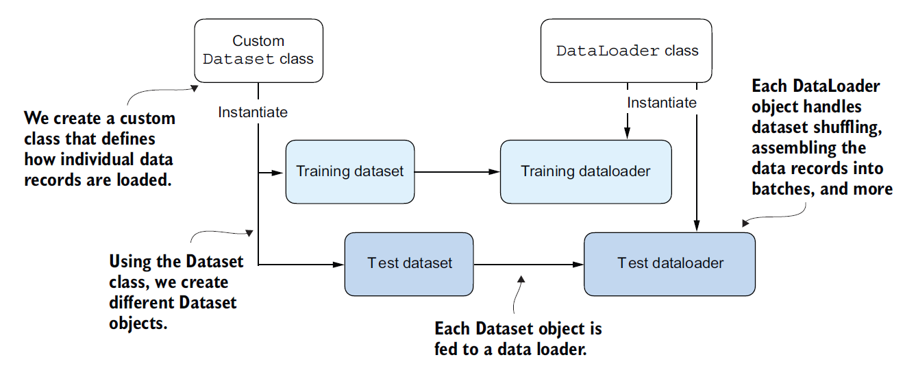
PyTorch implements a Dataset class and a DataLoader class. The Dataset class is used to create objects that define how each data record is loaded. The DataLoader handles how the data is shuffled and assembled into batches. Source: Raschka (2024).

A toy dataset with Dataset and DataLoader

X_train = torch.tensor([
    [-1.2, 3.1],
    [-0.9, 2.9],
    [-0.5, 2.6],
    [2.3, -1.1],
    [2.7, -1.5]
])

y_train = torch.tensor([0, 0, 0, 1, 1])

X_test = torch.tensor([
    [-0.8, 2.8],
    [2.6, -1.6]
])

y_test = torch.tensor([0, 1])

Note: PyTorch requires class labels to start at label 0, and the largest class label value must not exceed the number of output nodes minus 1 (since Python indexing starts at zero). So if we have class labels 0, 1, 2, 3 and 4, the output layer of the neural network should have five nodes.

In PyTorch, the three main components of a custom Dataset class are the __init__ constructor, the __getitem__ method and the __len__ method.

• In the __init__ method, we set up attributes that we can access later in the __getitem__ and __len__ methods. These could be file paths, file objects, database connectors, and so on.

• In the __getitem__ method, we define the instructions for returning exactly one item from the dataset via an index. This refers to the features and class label of a single training example or test instance.

• Finally, the __len__ method contains the instructions for retrieving the length of the dataset. Here, we use a tensor’s .shape attribute to return the number of rows in the feature array.

from torch.utils.data import Dataset, DataLoader

class ToyDataset(Dataset):
    def __init__(self, X, y):
        self.features = X
        self.labels = y
    
    # Instructions for retrieving exactly one data record and the corresponding label
    def __getitem__(self, index):
        one_x = self.features[index]
        one_y = self.labels[index]
        return one_x, one_y
    
    # Instructions for returning the length of the dataset
    def __len__(self):
        return self.labels.shape[0]
    

train_ds = ToyDataset(X_train, y_train)
test_ds = ToyDataset(X_test, y_test)

print(len(train_ds))

5

from torch.utils.data import DataLoader

torch.manual_seed(123)

# The ToyDataset insatance created earlier serves aas input in the data loader
train_loader = DataLoader(
    dataset=train_ds,
    batch_size=2,
    shuffle=True, # Wether or not to shuffle the data
    num_workers=0 # The number of background processes
)

test_loader = DataLoader(
    dataset=test_ds,
    batch_size=2,
    shuffle=False, # It is not necessary to shuffle a test dataset
    num_workers=0
)

shuffle=True shuffles the order of the examples at every training epoch. Its main purpose is to keep the model from learning a bias tied to the order of the data. In practice, it helps optimization with SGD/minibatches, makes training more stable, and often improves generalization.

It is mostly used during training, because the model should see the examples in a different order on each pass. If the data is ordered by class, difficulty, time or source, not shuffling can make training worse.

It is generally not used during testing or validation, because we want a deterministic, reproducible evaluation. The order of the examples should not influence the performance measurement. So we keep shuffle=False to test, validate and compare results consistently.

A case to watch out for: if your data is sequential or temporal, like a time series or some language problems, shuffling certain elements can be wrong. In that case, a different kind of splitting or batching is used.

In summary:

• training: usually shuffle=True
• validation/test: almost always shuffle=False
• exception: sequential or order-dependent data

for idx, (x, y) in enumerate(train_loader):
    print(f"Batch {idx + 1}: ", x, y)

Batch 1:  tensor([[ 2.3000, -1.1000],
        [-0.9000,  2.9000]]) tensor([1, 0])
Batch 2:  tensor([[-1.2000,  3.1000],
        [-0.5000,  2.6000]]) tensor([0, 0])
Batch 3:  tensor([[ 2.7000, -1.5000]]) tensor([1])

As the output above shows, train_loader goes through the training dataset, visiting each example exactly once. This is called a training epoch.

Since we seeded the random generator with torch.manual_seed(123) here, you should get exactly the same shuffle order for the training examples. However, if you iterate over the dataset a second time, you will see that the shuffle order changes.

This is intentional, to keep deep neural networks from getting stuck in repetitive update cycles during training.

We specified a batch size of 2 here, but the third batch contains only one example. That is because we have five training examples, and 5 is not evenly divisible by 2.

In practice, having a considerably smaller last batch in a training epoch can disturb convergence during training. To prevent this, set drop_last=True, which drops the last batch of each epoch, as shown in the following listing.

train_loader = DataLoader(
    dataset=train_ds,
    batch_size=2,
    shuffle=True,
    num_workers=0,
    drop_last=True
)

for idx, (x, y) in enumerate(train_loader):
    print(f"Batch {idx}:", x, y)

Batch 0: tensor([[-1.2000,  3.1000],
        [-0.5000,  2.6000]]) tensor([0, 0])
Batch 1: tensor([[ 2.3000, -1.1000],
        [-0.9000,  2.9000]]) tensor([1, 0])

Deep learning relies on a subtle marriage between high-level software abstractions and a fine understanding of the underlying computer hardware. When an engineer writes DataLoader(dataset, num_workers=4, batch_size=32), they are in fact mobilizing a whole ecosystem involving system processes, inter-process communication mechanisms, memory hierarchies, and compute units with radically different architectures.

As a beginner, it is only natural to wonder: how does data travel from disk storage to the compute cores of a GPU, and how can this pipeline be optimized when several processing units are available?

That is what we will try to answer in the following sections.

Under the hood: the DataLoader and its workers

The training loop and its fundamental bottleneck

A neural network trains through successive iterations. At each iteration, the model receives a batch of data, computes a prediction (forward pass), measures its error with a loss function, then backpropagates this error through its layers to adjust its parameters (backward pass). This sequence repeats thousands, even millions, of times.

This loop, however, has an asymmetric time structure: the GPU, when running a forward and backward pass, works at considerable speed, on the order of a few milliseconds per batch on modern hardware. By contrast, loading that batch from disk, decoding it, applying transformations and assembling it into a tensor can take a comparable time, or even longer. If these two phases run sequentially (that is, if the GPU waits for the data to be ready before starting to compute), then the GPU is actually idle half the time. This is called an I/O bottleneck. For equipment that costs several thousand euros, that waste is unacceptable.

The conceptual solution is a pipeline: prepare the next batches while the GPU works on the current one. This is exactly what the workers mechanism does.

Internal architecture of the DataLoader

PyTorch’s DataLoader is not a simple iterator. It is an orchestrator that coordinates several distinct components, each with a precise responsibility.

The Dataset is the abstraction layer that represents the data. It exposes a minimal interface: __len__() to know the number of items, and __getitem__(i) to access the item at index i. All the loading logic lives in this method: opening files, decoding images, reading from a database, and so on. The Dataset is deliberately unaware of batches: it works on individual samples.

The Sampler is responsible for defining the order in which the indices are visited. The SequentialSampler goes through them in natural order (0, 1, 2, …, N-1). The RandomSampler, enabled by shuffle=True, generates a random permutation of these indices at each new epoch. This randomization is crucial for training: it keeps the model from memorizing the order of the data and improves generalization.

The BatchSampler is a layer on top of the Sampler. It groups the indices generated by the Sampler into sublists of size batch_size. If drop_last=True, the last group is dropped when it contains fewer than batch_size items.

The collate_fn is the function that, given a list of individual samples, assembles them into a batch of tensors. By default, PyTorch provides a collate_fn that stacks the individual tensors along a new axis at dimension zero. You can provide a custom function to handle complex data structures (dictionaries, variable-size objects, and so on).

The workers are the child processes that run dataset[i] and apply the transformations, in parallel with the main process.

num_workers=0 mode: everything in the main process

When num_workers=0 (the default), there are no child processes. The main process is alone, and it performs every operation sequentially:

[Main Process]
  1. Ask the BatchSampler for the indices → [3, 1]
  2. Call dataset[3] → load and decode sample 3
  3. Call dataset[1] → load and decode sample 1
  4. Call collate_fn([sample_3, sample_1]) → batch
  5. Transfer the batch to the GPU
  6. Run the forward pass
  7. Run the backward pass
  8. Update the weights
  9. Go back to 1.

In this mode, the GPU is idle during steps 1 to 5. It waits for the CPU to finish preparing the data.

This mode is nonetheless perfectly suited to small datasets fully loaded into RAM (as in our toy example with 5 tensors), because the loading cost is negligible and workers would add pointless startup overhead.

num_workers > 0 mode: process-based parallelism

As soon as num_workers=N with N > 0, PyTorch creates N child processes when iteration starts. These processes are created through the fork mechanism (or spawn on Windows and macOS, depending on the configuration), a system call that duplicates the parent process’s memory space.

The control flow then becomes:

[Main Process]
  ├── Creates N workers at startup
  ├── Generates the index groups through the BatchSampler
  ├── Puts these groups in the Index Queue
  ├── Waits for a batch to appear in the Result Queue
  └── As soon as a batch arrives → GPU forward/backward → update

[Worker 1]
  ├── Waits for a group of indices to become available
  ├── Takes, for example, [0,1,2,3] from the Index Queue
  ├── Loads dataset[0], dataset[1], ...
  ├── Applies the transforms
  ├── Builds the batch with collate_fn
  └── Puts the batch in the Result Queue

[Worker 2]
  ├── Takes another group of indices
  └── Does the same work in parallel

The workers communicate with the main process through two shared queues:

• Index Queue: holds the groups of indices to process;
• Result Queue: holds the batches that are already prepared.

These queues are multiprocessing.Queue objects, designed specifically to let several independent processes communicate safely.

The key point is that several workers can access the same queue without getting in each other’s way. When a worker runs:

indices = index_queue.get()

the operation is automatically protected by an internal synchronization mechanism (a lock). This guarantees that only one worker can take a given item.

For example, if the queue contains:

[[0,1], [2,3], [4,5], [6,7]]

and two workers ask for work at the same moment:

• Worker 1 gets [0,1]
• Worker 2 gets [2,3]

Once a group of indices has been taken, it disappears from the queue immediately. No other worker can therefore receive the same group.

After retrieving its indices, each worker:

1. loads the corresponding examples with dataset[i],
2. applies any transformations,
3. groups the data with collate_fn,
4. then puts the final batch in the Result Queue.

Meanwhile, the main process keeps training on the GPU. As soon as it finishes a batch, it immediately picks up the next one from the Result Queue.

To make these exchanges fast, PyTorch uses shared memory. Without it, each batch would have to be copied in full from one process to another, which would cost a lot of time and memory.

Instead:

• the tensors are placed in a memory region accessible to all processes;
• the queue mostly passes a reference to that shared memory region.

This way, large data is not needlessly copied between the workers and the main process.

The prefetch_factor parameter controls how many batches each worker prepares in advance.

For example:

num_workers = 4
prefetch_factor = 2

means that:

• each worker can prepare up to 2 pending batches;
• so up to 4 × 2 = 8 batches can be ready or in preparation at the same time.

The idea is that the GPU should almost never have to wait for data: while it trains the model on one batch, the workers are already preparing the next ones in the background.

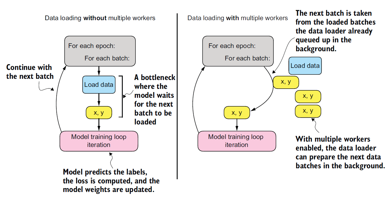
Loading data without multiple workers (setting num_workers=0) will create a data loading bottleneck where the model sits idle until the next batch is loaded (left). If multiple workers are enabled, the data loader can queue up the next batch in the background (right). Source: Raschka (2024).

The pin_memory mechanism

So far, the optimization has mainly concerned communication between the different CPU processes. Thanks to shared memory, the workers can efficiently hand the prepared batches over to the main process without needlessly copying tensors in memory.

However, once the main process has retrieved the batch, a second critical step begins: transferring the data from RAM to the graphics card’s memory (VRAM). This communication between the CPU and the GPU has its own hardware constraints and can quickly become a bottleneck too.

In other words, the full pipeline now looks like this:

CPU workers ──(shared memory)──> CPU main process ──(?)──> GPU

Shared memory therefore only optimizes the first link, the one between the CPU processes. It does not directly speed up the transfer of data to the GPU. The pinned memory mechanism, enabled with pin_memory=True, exists precisely to optimize this second link.

To understand why it is useful, we first need to distinguish a computer’s two main kinds of memory:

• the hard drive (or SSD), very large but relatively slow;
• main memory (RAM), much faster but with more limited capacity.

When RAM starts to fill up, the operating system uses a mechanism called virtual memory (or swapping). Some data that is temporarily little used can then be moved from RAM to the hard drive to free up memory.

For ordinary applications, this mechanism is extremely convenient and completely transparent. But when training a neural network on a GPU, this flexibility becomes a problem.

During training:

1. the CPU prepares the batches in RAM;
2. then the GPU has to fetch this data to run the computations.

The GPU, however, behaves like an extremely fast device that needs the data to stay physically in place in memory during the transfer. If the operating system suddenly moved part of the batch to the hard drive at the wrong moment, the transfer would become much slower.

This is exactly what pin_memory=True is for.

When this option is enabled, PyTorch asks the operating system to place the batches in a special region of RAM called pinned memory (page-locked memory). This memory is “locked”:

• the operating system is no longer allowed to move this data to disk;
• the data stays physically fixed in RAM during the transfer.

The GPU can then access this memory directly through a hardware mechanism called DMA (Direct Memory Access).

The transfer therefore becomes:

Pinned RAM ──(fast DMA)──> GPU VRAM

The benefit is twofold:

1. the CPU → GPU transfer becomes much faster;
2. the CPU no longer needs to constantly supervise the copy and can already start preparing the next batch.

The pipeline then becomes much smoother:

[CPU workers]
      │
      ├── Prepare the batches
      │
      ├── Shared Memory
      │
      ▼
[CPU main process]
      │
      ├── pin_memory: locks the batch in RAM
      │
      ▼
[GPU]
      ├── Fetches the data through DMA
      └── Runs the training

Without pin_memory=True, the transfer is less efficient. Since the data lives in “normal” RAM (pageable memory), the system often has to perform an extra intermediate step:

1. copy the data to a temporarily locked region;
2. only then start the transfer to the GPU.

This extra copy needlessly ties up the CPU and slows down the whole training pipeline.

So:

• shared memory optimizes exchanges between CPU processes;
• pinned memory optimizes transfers between RAM and the GPU.

These two mechanisms therefore come into play at different but complementary stages of the data loading pipeline.

A Typical Training Loop

Now let’s train the neural network on the toy dataset

import torch.nn.functional as F

torch.manual_seed(123)
model = NeuralNetwork(num_inputs=2, num_outputs=2) # The dataset has two features and two classes
optimizer = torch.optim.SGD(
    model.parameters(), lr=0.5 # The optimizer needs to know which parameters to optimize
)
num_epochs = 3
for epoch in range(num_epochs):
    model.train()
    for batch_idx, (features, labels) in enumerate(train_loader):
        # Forward pass
        logits = model(features)
        loss = F.cross_entropy(logits, labels)

        # Backward pass
        optimizer.zero_grad() # Sets the gradients from the previous round to 0 to prevent unintended gradient accumulation
        loss.backward() # Computes the gradients of the loss given the model parameters
        optimizer.step() # The optimizer uses the gradients to update the model parameters 

        ### LOGGING
        print(f"Epoch: {epoch+1:03d}/{num_epochs:03d}"
              f" | Batch {batch_idx:03d}/{len(train_loader):03d}"
              f" | Train Loss: {loss: .2f}")
        
    model.eval()
    # Insert optional model evaluation code 

Epoch: 001/003 | Batch 000/002 | Train Loss:  0.75
Epoch: 001/003 | Batch 001/002 | Train Loss:  0.65
Epoch: 002/003 | Batch 000/002 | Train Loss:  0.44
Epoch: 002/003 | Batch 001/002 | Train Loss:  0.13
Epoch: 003/003 | Batch 000/002 | Train Loss:  0.03
Epoch: 003/003 | Batch 001/002 | Train Loss:  0.00

# Exercise A.3 :
num_params = sum(p.numel() for p in model.parameters() if p.requires_grad)
print("Total number of trainable model parameters:", num_params)

Total number of trainable model parameters: 752

In practice, we often use a third dataset, called a validation dataset, to find the optimal hyperparameter settings.

We have also introduced new settings called model.train() and model.eval(). As their names suggest, these settings put the model into a training mode and an evaluation mode. This is needed for components that behave differently during training and inference, such as dropout or batch normalization layers.

Since our NeuralNetwork class has no dropout or other components affected by these settings, using model.train() and model.eval() is redundant in our code above. However, it is good practice to include them anyway, to avoid unexpected behavior when we change the model architecture or reuse the code to train a different model.

As discussed earlier, we pass the logits directly to the cross_entropy loss function, which applies the softmax function internally for efficiency and numerical stability.

Then, calling loss.backward() computes the gradients in the computation graph that PyTorch built in the background. The optimizer.step() method uses the gradients to update the model parameters so as to minimize the loss.

With the SGD optimizer, this means multiplying the gradients by the learning rate and adding the scaled negative gradient to the parameters.

Why pass the logits directly to the cross-entropy?

In PyTorch, we usually pass the logits (raw outputs) directly to the cross_entropy loss function, without applying Softmax ourselves, for reasons of numerical stability.

1. The problem (numerical instability)

If a model produces a very large logit, computing the softmax ($e^x$) by hand causes a memory overflow.

Naive example:

import torch

logits = torch.tensor([1000.0, 2.0, -1.0])
exponentials = torch.exp(logits) 
# Result: tensor([inf, 7.3891, 0.3679])  <-- The computer cannot handle e^1000

probabilities = exponentials / torch.sum(exponentials)
# Result: tensor([nan,  0.,  0.])  <-- inf/inf breaks the computation (Not a Number)

2. The solution (what PyTorch does behind the scenes)

PyTorch uses the LogSumExp mathematical trick. Before computing the exponential, it subtracts the maximum value from all the logits.

The trick in action:

# Subtract the maximum (1000) from all the logits
stable_logits = logits - torch.max(logits)
# Result (1000-1000, 2-1000, -1-1000): tensor([0., -998., -1001.])

stable_exponentials = torch.exp(stable_logits)
# Result: tensor([1.0, 0.0, 0.0])  <-- No more "inf"! The exponential of 0 is 1.

3. Why does the subtraction give the same probabilities? (The proof)

You might think that changing the logits distorts the final result. But the softmax function is insensitive to adding or subtracting a constant! Here is the mathematical proof:

The probability formula for a logit $x_i$ is:

If we subtract a constant $C$ (our maximum) from all the logits, the power rule ($e^{a-b} = e^a \times e^{-b}$) gives:

Since $e^{-C}$ appears in every term of the sum in the denominator, we can factor it out:

The term $e^{-C}$ appears at the top and bottom of the fraction, so it cancels out:

Conclusion: Subtracting the maximum changes the intermediate numbers to avoid the memory crash, but the final division restores the balance. By passing the logits directly to cross_entropy, PyTorch performs this complex optimization in a single, ultra-fast block.

Making predictions and measuring accuracy

# After we have trained the model, we can use it to make predictions
model.eval()
with torch.no_grad():
    outputs = model(X_train)
print(outputs)

tensor([[ 2.8569, -4.1618],
        [ 2.5382, -3.7548],
        [ 2.0944, -3.1820],
        [-1.4814,  1.4816],
        [-1.7176,  1.7342]])

To get the class membership probabilities, we can then use PyTorch’s softmax function

torch.set_printoptions(sci_mode=False)
probas = torch.softmax(outputs, dim=1)
print(probas)

tensor([[0.9991, 0.0009],
        [0.9982, 0.0018],
        [0.9949, 0.0051],
        [0.0491, 0.9509],
        [0.0307, 0.9693]])

The call to set_printoptions is used here to make the output easier to read.

By default, if the numbers in your tensors are very small or very large, PyTorch uses scientific notation (for example 1.234e-05 instead of 0.000012).

# We can convert these values into class label predictions
predictions = torch.argmax(probas, dim=1)
print(predictions)

tensor([0, 0, 0, 1, 1])

Note that we don’t need to compute the softmax probabilities to get the class labels. We could also apply the argmax function directly to the logits.

predictions = torch.argmax(outputs, dim=1)
print(predictions)

tensor([0, 0, 0, 1, 1])

Since the training dataset is relatively small, we could compare the predicted labels with the true labels by eye.

predictions == y_train

tensor([True, True, True, True, True])

Using torch.sum, we can count the number of correct predictions.

torch.sum(predictions == y_train)

tensor(5)

To generalize the computation of the prediction accuracy, let’s implement the compute_accuracy function

def compute_accuracy(model, dataloader):

    model.eval()
    correct = 0.0
    total_examples = 0

    for idx, (features, labels) in enumerate(dataloader):

        with torch.no_grad():
            logits = model(features)

        predictions = torch.argmax(logits, dim=1)
        # Returns a tensor of True/False values depending on whether the labels match
        compare = labels == predictions
        # The sum operations counts the number of True values
        correct += torch.sum(compare)
        total_examples += len(compare)

    # The fraction of correct prediction, a value between 0 and 1.
    # item() returns the value of the tensor as Python float.
    return (correct / total_examples).item()

# We can then apply the function to the training 
print(compute_accuracy(model, train_loader))

1.0

# Similary, we can apply the function to the test set
print(compute_accuracy(model, test_loader))

1.0

Saving and Loading Models

# To save models in Pytorch
torch.save(model.state_dict(), "model.pth")

The model’s state_dict is a Python dictionary object that maps each layer of the model to its trainable parameters (weights and biases).

model.pth is an arbitrary file name for the model file saved to disk. We can give it any name and file extension we like; however, .pth and .pt are the most common conventions.

# Once the model is saved, we can load it back from disk
model =  NeuralNetwork(2, 2)
model.load_state_dict(torch.load("model.pth"))

<All keys matched successfully>

The torch.load() function reads the model.pth file and rebuilds the Python dictionary object containing the model’s parameters, while model.load_state_dict() applies these parameters to the model, effectively restoring the state it had learned at the moment we saved it.

The line model = NeuralNetwork(2, 2) was included here to show that we need an instance of the model in memory to apply the saved parameters.

Optimizing Training Performance with GPUs

PyTorch Computations on GPU Devices

In PyTorch, a device is where computations take place and where data resides. The CPU and the GPU are examples of devices. A PyTorch tensor resides on a device, and its operations run on that same device.

# We can double-check that our runtime indeed supports GPU computing
print(torch.cuda.is_available())

True

Now suppose we have two tensors that we can add together; this computation runs on the CPU by default

tensor_1 = torch.tensor([1., 2., 3.])
tensor_2 = torch.tensor([4., 5., 6.])
print(tensor_1 + tensor_2)

tensor([5., 7., 9.])

We can now use the .to() method. It is the same method we used to change a tensor’s data type, but this time to transfer these tensors to a GPU and run the addition there.

tensor_1 = tensor_1.to("cuda")
tensor_2 = tensor_2.to("cuda")
print(tensor_1 + tensor_2)

tensor([5., 7., 9.], device='cuda:0')

The resulting tensor now includes the device information, device='cuda:0', which means that the tensors reside on the first GPU. If your machine hosts several GPUs, you can specify which GPU to transfer the tensors to. You do this by giving the device ID in the transfer command. For example, you can use .to(“cuda:0”), .to(“cuda:1”), and so on.

However, all the tensors must be on the same device. Otherwise, the computation will fail if one tensor resides on the CPU and the other on the GPU:

try:
    print(tensor_1 + tensor_2)
except RuntimeError as e:
    print(f"Error: {e}")

tensor([5., 7., 9.], device='cuda:0')

Training on a Single GPU

A training loop on a GPU

torch.manual_seed(123)
model = NeuralNetwork(num_inputs=2, num_outputs=2)

# Defines a device varaible that defaults to a GPU
device = torch.device("cuda")
# Transfers the model onto the GPU
model = model.to(device)

optimizer = torch.optim.SGD(model.parameters(), lr=0.5)

num_epochs = 3

for epoch in range(num_epochs):
    model.train()
    for batch_idx, (features, labels) in enumerate(train_loader):
        # Transfers the data onto the GPU
        features, labels = features.to(device), labels.to(device)
        logits = model(features)
        loss = F.cross_entropy(logits, labels) # Loss function

        optimizer.zero_grad()
        loss.backward()
        optimizer.step()

        ### LOGGING
        print(f"Epoch: {epoch+1:03d}/{num_epochs:03d}"
              f" | Batch {batch_idx:03d}/{len(train_loader):03d}"
              f" | Train/ Val Loss: {loss: .2f}")

    model.eval()
    # Insert optional model evaluation code

Epoch: 001/003 | Batch 000/002 | Train/ Val Loss:  0.75
Epoch: 001/003 | Batch 001/002 | Train/ Val Loss:  0.65
Epoch: 002/003 | Batch 000/002 | Train/ Val Loss:  0.44
Epoch: 002/003 | Batch 001/002 | Train/ Val Loss:  0.13
Epoch: 003/003 | Batch 000/002 | Train/ Val Loss:  0.03
Epoch: 003/003 | Batch 001/002 | Train/ Val Loss:  0.00

The role of .to(device): triggering the transfer to the GPU

At this point, the CPU pipeline is fully optimized:

• the workers built the batch in shared memory;
• the Result Queue passed the main process a reference to that memory region, not a copy of the data;
• if pin_memory=True, the batch is already locked in a stable region of RAM, ready for a DMA transfer.

Yet none of this has sent anything to the GPU yet. The batch only exists in RAM. The GPU can only run computations on data residing in its own memory (VRAM): it cannot access the CPU’s RAM directly for every operation.

This is exactly what the following line explicitly triggers:

features, labels = features.to(device), labels.to(device)

This instruction tells PyTorch to allocate a block in VRAM and copy the tensor’s numerical values into it from RAM. Without pin_memory, this copy requires an intermediate step on the CPU side. With pin_memory=True, the transfer happens directly through DMA, without the CPU getting involved.

The complete pipeline is therefore:

[Disk]
      │  read files
      ▼
[CPU workers]
      │  transforms + collate_fn → tensor in shared memory
      ▼
[Result Queue]
      │  passes a reference to the shared memory (not a copy)
      ▼
[CPU main process]
      │  accesses the batch through the reference
      │  (pin_memory: batch already in locked RAM)
      ▼
[.to(device)]
      │  triggers the RAM → VRAM transfer
      │  (through DMA if pin_memory=True)
      ▼
[GPU / VRAM]
      └── forward / backward / weight update

One more constraint makes this transfer mandatory: PyTorch requires all operations to involve tensors on the same device. Since the model was placed in VRAM with model.to(device), any data passed to it must be there too, or PyTorch immediately raises a runtime error.

So .to(device) is not a minor technical detail. It is the last link in the loading pipeline, the one that makes the data actually usable by the GPU for computation.

Batch ordering and GPU processing

The previous sections showed how the workers prepare batches in parallel. A question then naturally arises: in what order does the GPU process these batches, given that several workers progress at the same time and do not necessarily finish at the same moment?

Workers do not finish in a predictable order.

Although all the workers start their processing in parallel, their execution time is not uniform. Two main factors introduce differences:

• the scheduler (the operating system component that decides which process gets to use the CPU at a given moment) does not allocate compute time in a strictly fair way. Other system processes can slip in, temporarily suspend a worker and delay its progress regardless of the work it is doing;
• disk access can be uneven, especially on a mechanical hard drive (HDD), where a physical read head moves to reach the files. If a batch’s examples are scattered across the disk, this movement takes longer than for files that sit physically close together. On an SSD this factor is smaller, but contention remains when several workers read at the same time and compete for read bandwidth.

It is therefore quite possible for the worker handling batch #2 to finish before the one handling batch #0.

PyTorch nevertheless guarantees batch order.

To keep the order deterministic, PyTorch attaches a sequence number to each group of indices when the BatchSampler generates it:

BatchSampler generates:
  batch #0 → indices [0,1,2,3]
  batch #1 → indices [4,5,6,7]
  batch #2 → indices [8,9,10,11]

This number travels with the batch throughout its processing. When the workers drop their results into the Result Queue, it can therefore receive the batches in any order:

Result Queue (actual arrival order):
  (number=2, batch_2)
  (number=0, batch_0)
  (number=1, batch_1)

The main process never simply takes the first available batch. It waits specifically for the next expected sequence number. Batches that arrive early are kept in an internal buffer until their turn comes:

Main process waits for #0:
  → batch #2 arrives → put in the buffer
  → batch #0 arrives → sent to the GPU  ✅

Main process waits for #1:
  → batch #1 arrives → sent to the GPU  ✅

Main process waits for #2:
  → batch #2 already in the buffer → sent to the GPU  ✅

The GPU processes batches sequentially.

A standard GPU processes only one batch at a time. The parallelism of the workers is therefore not meant to feed several GPU computations at once: its only purpose is to eliminate the GPU’s waiting time between two batches. Without workers, the GPU would sit idle for as long as it takes to prepare the next batch. With several workers, that batch is already waiting in the Result Queue before the GPU even needs it.

The complete pipeline can therefore be summarized as:

[Workers in parallel]
  W1: batch #1 ──┐
  W2: batch #0 ──┼──> Result Queue (any order)
  W3: batch #2 ──┘           │
                             │ 
                        reordering 
                     by sequence number
                             |
                             |
                             ▼
           [Main Process] → [GPU]: #0 → #1 → #2 → ...
                                   (guaranteed order, continuous flow)

The parallelism is therefore entirely on the CPU preparation side. The GPU remains a sequential consumer, but one that almost never runs out of data thanks to the batches prepared in advance by the workers.

Note: Buffer literally means a temporary waiting area in memory.

In this specific context, it is simply a Python dictionary that PyTorch maintains in the main process, where it stores batches received “too early” until their sequence number comes up.

Concretely:

Main process waits for number #0.

→ batch #2 arrives first in the Result Queue.
  The main process picks it up, sees that it is #2,
  and stores it in the buffer:
  buffer = { 2: batch_2 }

→ batch #0 finally arrives.
  It is the right number → sent to the GPU immediately.
  buffer = { 2: batch_2 }  ← still there, waiting its turn

→ Main process now waits for #1.
  batch #1 arrives → sent to the GPU.

→ Main process waits for #2.
  Already in the buffer → picked up directly, sent to the GPU.
  buffer = {}  ← emptied

The buffer avoids rejecting or ignoring a batch that arrives early: it simply keeps it in RAM until the right moment. It is just a waiting structure, nothing more.

We can use .to("cuda") instead of device = torch.device("cuda"). Transferring a tensor to cuda instead of torch.device("cuda") also works and is shorter.

We can also modify the statement so that the same code runs on a CPU if no GPU is available. This is considered good practice when sharing PyTorch code:

device = torch.device("cuda" if torch.cuda.is_available() else "cpu")

On an Apple Mac with an Apple Silicon chip (such as the M1, M2, M3 or newer models) instead of a computer with an Nvidia GPU, you can change

device = torch.device("cuda" if torch.cuda.is_available() else "cpu")

to

device = torch.device("mps" if torch.backends.mps.is_available() else "cpu")

Exercise A.4: CPU or GPU, which is faster?

Compare the execution time of matrix multiplication on a CPU with that on a GPU.

At what matrix size do you start to see matrix multiplication on the GPU run faster than on the CPU? Hint: use the %timeit command in Jupyter to compare execution times. For example, given matrices a and b, run the command %timeit a @ b in a new notebook cell.

size = 32

import torch
size = (32, 32)
# Matrices on the CPU
a_cpu = torch.randn(size)
b_cpu = torch.randn(size)

# The same matrices transferred to the GPU
a_gpu = a_cpu.to("cuda")
b_gpu = b_cpu.to("cuda")

%timeit a_cpu @ b_cpu

6.1 µs ± 1.17 µs per loop (mean ± std. dev. of 7 runs, 100000 loops each)

%timeit a_gpu @ b_gpu

15 µs ± 1.57 µs per loop (mean ± std. dev. of 7 runs, 100000 loops each)

size = 64

import torch
size = (64, 64)
# Matrices on the CPU
a_cpu = torch.randn(size)
b_cpu = torch.randn(size)

# The same matrices transferred to the GPU
a_gpu = a_cpu.to("cuda")
b_gpu = b_cpu.to("cuda")

%timeit a_cpu @ b_cpu

8.51 µs ± 217 ns per loop (mean ± std. dev. of 7 runs, 100000 loops each)

%timeit a_gpu @ b_gpu

14.3 µs ± 1.86 µs per loop (mean ± std. dev. of 7 runs, 100000 loops each)

size = 128

import torch
size = (128, 128)
# Matrices on the CPU
a_cpu = torch.randn(size)
b_cpu = torch.randn(size)

# The same matrices transferred to the GPU
a_gpu = a_cpu.to("cuda")
b_gpu = b_cpu.to("cuda")

%timeit a_cpu @ b_cpu

54 µs ± 12.5 µs per loop (mean ± std. dev. of 7 runs, 10000 loops each)

%timeit a_gpu @ b_gpu

13.3 µs ± 1.14 µs per loop (mean ± std. dev. of 7 runs, 100000 loops each)

size = 256

import torch
size = (256, 256)
# Matrices on the CPU
a_cpu = torch.randn(size)
b_cpu = torch.randn(size)

# The same matrices transferred to the GPU
a_gpu = a_cpu.to("cuda")
b_gpu = b_cpu.to("cuda")

%timeit a_cpu @ b_cpu

276 µs ± 6.94 µs per loop (mean ± std. dev. of 7 runs, 1000 loops each)

%timeit a_gpu @ b_gpu

21.7 µs ± 247 ns per loop (mean ± std. dev. of 7 runs, 10000 loops each)

size = 512

import torch
size = (512, 512)
# Matrices on the CPU
a_cpu = torch.randn(size)
b_cpu = torch.randn(size)

# The same matrices transferred to the GPU
a_gpu = a_cpu.to("cuda")
b_gpu = b_cpu.to("cuda")

%timeit a_cpu @ b_cpu

2.04 ms ± 100 µs per loop (mean ± std. dev. of 7 runs, 100 loops each)

%timeit a_gpu @ b_gpu

64.5 µs ± 196 ns per loop (mean ± std. dev. of 7 runs, 10000 loops each)

size = 1024

import torch
size = (1024, 1024)
# Matrices on the CPU
a_cpu = torch.randn(size)
b_cpu = torch.randn(size)

# The same matrices transferred to the GPU
a_gpu = a_cpu.to("cuda")
b_gpu = b_cpu.to("cuda")

%timeit a_cpu @ b_cpu

16.8 ms ± 2.65 ms per loop (mean ± std. dev. of 7 runs, 100 loops each)

%timeit a_gpu @ b_gpu

603 µs ± 3.74 µs per loop (mean ± std. dev. of 7 runs, 1000 loops each)

Multi-GPU training: strategies and mechanisms

Why several GPUs?

To understand why several GPUs are useful, you first need to grasp two fundamental and quite distinct limits that come up when training modern models.

The first limit is a physical storage limit. Each GPU has video memory (VRAM) with a fixed, non-expandable capacity: typically between 16 GB and 80 GB on high-end models. Yet a large language model like GPT-3 weighs 350 GB on its own in float16 precision. It is therefore simply impossible, in the physical sense, to fit all of its parameters on a single GPU. No matter how fast the hardware is, the problem is not speed but capacity: you cannot fit a five-meter piece of furniture into a two-meter room. The model itself must be distributed across several GPUs, each hosting only a fraction of it.

The second limit is a time limit. Even when the model fits comfortably on a single GPU, training can take weeks or months. Here, the issue is no longer capacity but speed. With N GPUs able to process data in parallel, training time can theoretically be divided by N by processing N times more examples at any given moment.

These two motivations, one a hard constraint, the other an optimization, give rise to two major families of strategies that we will explore: data parallelism, where the model is duplicated and the data is split up; and model parallelism, where the model itself is split across the GPUs.

DataParallel (DP): the first, naive approach

torch.nn.DataParallel is PyTorch’s original API for multi-GPU training. To really understand its limits, you first need to understand how it works inside, which starts with two fundamental notions: what a process is and what a thread is.

Processes and threads: laying the groundwork.

When you launch a Python program, the operating system creates a process. This process is a fully autonomous, isolated unit of execution: it has its own memory space, its own resources, its own identity. Two processes share nothing by default. If one crashes, the other keeps running unaffected.

A thread is something finer-grained. It is a secondary line of execution that lives inside a single process. Several threads coexist in the same process, share the same memory space and resources, but each moves through the code at its own pace.

The most telling analogy is an office and its employees. The process is the office: it has its own walls, its own files, its own equipment. The threads are the employees working in that office. They all have access to the same cabinets, the same files, the same tools. It is precisely this sharing that lets them collaborate quickly, without having to exchange copies of documents. But the same sharing creates a risk: if two employees edit the same file at the same time, the result will be corrupted.

This is exactly the corruption Python’s GIL (Global Interpreter Lock) was introduced to prevent. Imagine there is only one pen in the office, and an employee must hold it to be allowed to act. The others can wait, observe, get ready, but they cannot execute anything until the pen is free. A direct and counterintuitive consequence: even if your machine has 8 physical cores able to run 8 threads of execution at once, Python will never let two threads truly run at the same time. One holds the pen, the others wait their turn. The apparent parallelism is therefore an illusion: it looks like simultaneous execution, but the threads actually take turns in very rapid alternation.

How DataParallel works.

DataParallel relies precisely on this thread model. To understand why that is a problem, let’s follow one training iteration.

The main process (a single office with a single boss) takes the whole batch from the DataLoader. It splits it into equal portions and hands one to each available GPU. Each GPU then runs an independent forward pass on its portion, in parallel. So far, the organization looks efficient.

But here is where the first problem shows up: once the computations are done on each GPU, all the outputs are sent back to GPU 0 so that it can gather them, compute the global loss, run the backward pass, then redistribute the gradients and resynchronize the weights of all the GPUs. In other words, the parallel work phase is short-lived: the rest of the iteration is entirely sequential and concentrated on a single device.

This model creates a structural bottleneck on GPU 0. It is the only one that receives the full batch, assembles the results, computes the global gradients and redistributes the weights. It is therefore constantly much busier than its peers. In practice, beyond 2 to 4 GPUs, additional GPUs bring almost no real gain: they spend most of their time waiting for GPU 0 to finish.

The second flaw: the GIL paralyzes coordination.

A second problem, less visible but just as costly, follows directly from the thread architecture described above. In DataParallel, the different GPUs are driven by separate Python threads, all living in the same process. The intention is good: to move several GPUs forward in parallel. But as soon as these threads need to run pure Python code (interpreting a loop, evaluating a condition, calling a custom function in the forward pass), they end up queuing in front of the GIL.

While GPU 0’s thread holds the pen, GPU 1’s thread is suspended, even though its GPU is physically available and eager to work. The more complex Python logic the model’s forward pass contains, the longer this queue gets, and the more the multi-GPU benefit evaporates. Coordination between threads, instead of speeding things up, ends up slowing them down.

These two flaws, the centralization on GPU 0 and the GIL, are not bugs that a patch can fix: they are the direct consequence of DataParallel’s founding architectural choice, a single process driving everything. That is the choice that had to be rethought, and that is exactly what DDP does.

DistributedDataParallel (DDP): today’s standard

To understand why DistributedDataParallel (DDP) is an architectural break rather than a simple improvement, we need to go back to the source of the previous problem: centralization. DataParallel had a single boss. DDP removes this hierarchy entirely.

From a centralized kitchen to a decentralized brigade.

With DDP, each GPU is managed by its own independent Python process, launched with torchrun. There is no longer a master process that everything converges on. Each process loads its own data, computes its own gradients and makes its own decisions, while staying perfectly synchronized with its peers. This independence between processes immediately solves the GIL problem, since we are now dealing with separate processes.

Each process loads its own data.

To keep all the GPUs from processing the same examples (which would be a total waste), PyTorch provides a DistributedSampler. Its role is to partition the dataset into disjoint subsets, one per process. With N processes and M examples in total, process number k is assigned the examples at indices k, k+N, k+2N, and so on. Together, the processes thus cover exactly the whole dataset, with no redundancy and nothing left out.

Synchronizing gradients with AllReduce.

At the end of the backward pass, each process has computed its own gradients, exact for its mini-batch but partial with respect to the whole dataset. For all the models to evolve identically and converge to the same solution, each GPU must apply the same update, that is, the average of the gradients computed across all the processes.

This is exactly what the AllReduce operation does. It guarantees that whichever GPU you ask, each one receives the complete sum (or average) of all the gradients computed by its peers. This operation is implemented by NCCL (NVIDIA Collective Communications Library), which uses the direct physical connections between GPUs: NVLink for GPUs on the same machine, InfiniBand or Ethernet for GPUs spread across remote servers.

The Ring-AllReduce algorithm: why a ring?

The naive way to implement AllReduce would be to send all the gradients to a central node that sums them and sends them back out. We would then fall back into DataParallel’s bottleneck. NCCL avoids this trap with Ring-AllReduce, whose elegance deserves an explanation.

Ring-AllReduce: how N GPUs exchange their gradients without a bottleneck

In distributed data-parallel training, each GPU computes its own gradients on its subset of the batch. They must then be averaged across all the GPUs before updating the weights. But the flaw is immediate: the central GPU has to receive the gradients from all the others, then send them back to all of them. Its communication load grows linearly with the number of GPUs. With a 300-million-parameter model (1.2 GB of gradients) and 10 GPUs, each iteration slows down by more than 10 seconds. The solution does not scale.

Ring-AllReduce removes this bottleneck by eliminating the central reducer. Here is how it works.

The topology. The N GPUs are arranged in a logical ring. Each GPU has exactly one neighbor on its left and one on its right. It only sends data to the right and only receives from the left.

The first phase: Scatter-Reduce. Each GPU splits its gradient array into N fragments of equal size. Then we go around the ring N-1 times. At each step, each GPU sends a fragment to its right-hand neighbor and receives a fragment from its left-hand neighbor, which it adds to its own corresponding fragment. The fragment sent at each step is always the one received at the previous step. After N-1 steps, each GPU holds one fragment containing the complete sum of that fragment, aggregated across all the GPUs. Not all the gradients: just its own portion, but fully reduced.

The second phase: Allgather. We go around the ring N-1 more times, but this time each GPU, instead of adding what it receives, simply overwrites the corresponding fragment with the received value. After N-1 steps, each GPU has successively received all the reduced fragments and therefore holds the complete aggregated gradients.

Why the bandwidth does not depend on N. At each step, each GPU sends and receives a fragment of size K/N (where K is the total size of the array). Over the 2(N-1) steps in total (N-1 per phase), the total amount of data transferred by each GPU is therefore 2(N-1) × K/N, which tends to 2K when N is large and, above all, does not depend on N. Whether there are 4 or 400 GPUs in the ring, each link carries the same amount of data. This is the fundamental property that makes the algorithm scalable: adding GPUs does not make communication worse.

The extra optimization. Since backpropagation computes gradients from the last layer to the first, the gradients of the output layers are available well before those of the input layers. We can therefore start the Ring-AllReduce on the first available gradients while the others are still being computed, overlapping communication and computation. In the paper’s experiments on a 300-million-parameter model, this saved 70 to 120 ms per iteration.

For more details, see Bringing HPC Techniques to Deep Learning.

Model Parallelism

As efficient as DDP is, it implicitly assumes one thing: that the model fits in the VRAM of a single GPU. When that is no longer the case (which is the norm for very large models), a completely different family of strategies is needed, in which it is no longer the dataset that is distributed, but the model itself.

Pipeline parallelism: the assembly line.

The most intuitive form of model parallelism assigns groups of layers to different GPUs. GPU 0 hosts the first layers, GPU 1 the next ones, and so on. During a forward pass, the activations are computed on GPU 0, passed to GPU 1 for the rest of the computation, then to GPU 2, and so on. The analogy with an industrial assembly line is direct: each station performs a specific operation and passes the result to the next one.

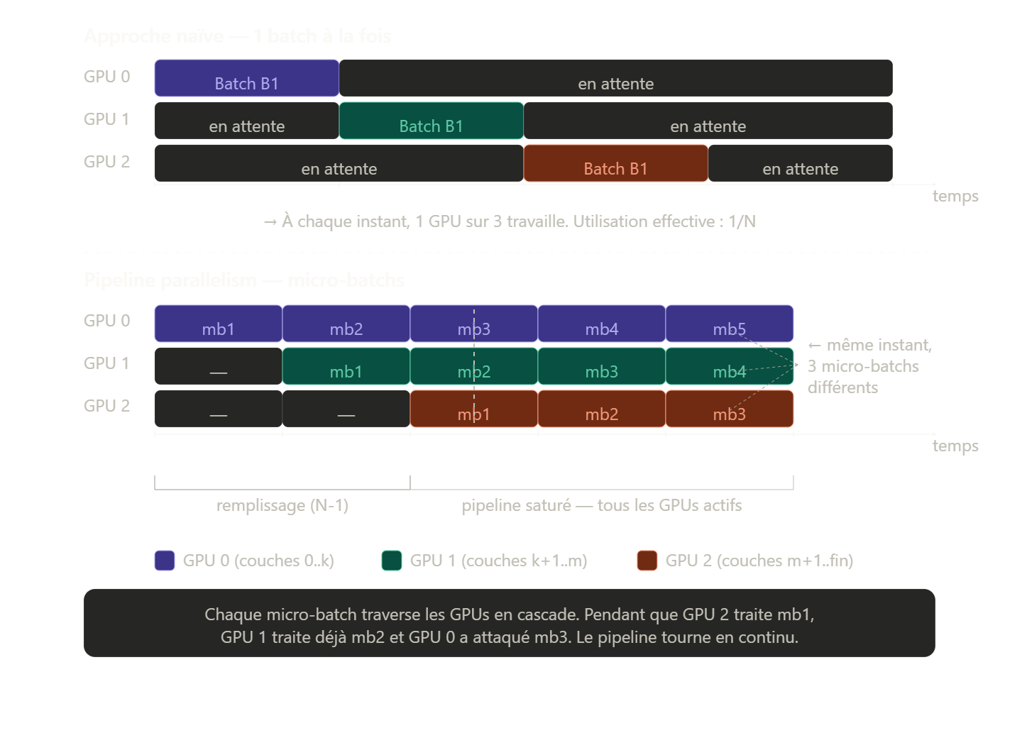
But this analogy also immediately reveals the major flaw of the naive approach. On a real assembly line where only one part moves at a time, every station is idle except one. This is exactly what happens here: at any given moment, only one GPU is working while all the others wait. The effective utilization is 1/N, which is catastrophic.

The solution is to stop sending a single batch through and instead split it into micro-batches fed into the pipeline in quick succession. As soon as GPU 0 has processed micro-batch 1 and passed it to GPU 1, it does not wait for the final result: it immediately starts on micro-batch 2. Meanwhile, GPU 1 receives micro-batch 1 and starts processing it. GPU 2 does the same one cycle later. The first cycles are spent filling the pipeline. This is unavoidable, like the start of any assembly line. But once the pipeline is full, all the GPUs work continuously, each on a different micro-batch at the same moment. This technique, introduced by GPipe and PipeDream, made training very large models economically viable.

Tensor parallelism: splitting the matrices themselves.

Pipeline parallelism distributes layers across GPUs, but what can be done when a single layer (a projection matrix in an attention mechanism, for example) is too large for one GPU on its own?

Tensor parallelism answers this question by distributing the weight matrices themselves across GPUs. Concretely, a large matrix can be split either by columns or by rows. Each GPU stores and computes only one fragment of the matrix, producing a partial result. These partial results are then aggregated through AllReduce to rebuild the complete output. This approach, popularized by NVIDIA’s Megatron-LM (see the paper Megatron-LM-Training Multi-Billion Parameter Language Models Using), therefore works within a single layer, whereas pipeline parallelism works between layers.

3D Parallelism: combining the three strategies.

In practice, large-scale models such as GPT-4 or LLaMA 3 do not choose between these strategies: they combine all three at once, in an arrangement called 3D Parallelism (see the paper Efficient Large-Scale Language Model Training on GPU Clusters Using Megatron-LM).

• Data parallelism (DDP) operates between groups of GPUs: several replicas of the same submodel process different mini-batches and synchronize their gradients.
• Pipeline parallelism operates between stages of layers: the different blocks of the model are spread across separate GPUs arranged in a cascade.
• Tensor parallelism operates within each layer: the matrices are split across the GPUs of the same stage.

Each dimension of this cube solves a different problem: tensor parallelism handles layers that are too wide, pipeline parallelism handles models that are too deep, and data parallelism maximizes throughput. Combining them is what makes it technically possible to train models with hundreds of billions of parameters on clusters of thousands of GPUs.

Other very interesting resources:

• How to Train Really Large Models on Many GPUs?
• The Ultra-Scale Playbook: Training LLMs on GPU Clusters

DDP in practice

DDP (Distributed DataParallel) enables parallelism by splitting the input data across the available devices and processing these data subsets at the same time.

PyTorch launches a separate process on each GPU, and each process receives and keeps a copy of the model; these copies are synchronized during training.

To illustrate this, suppose we have two GPUs that we want to use to train a neural network, as shown in the figure below:

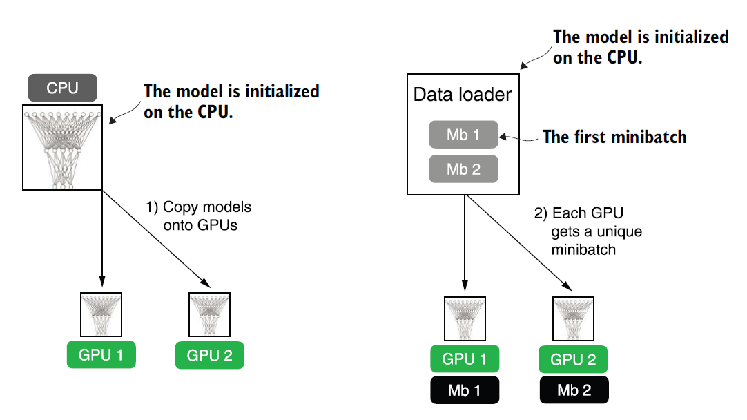
Transferring the model and data in DDP involves two key steps. First, we create a copy of the model on each GPU. Then, we split the input data into unique minibatches that we pass to each copy of the model. Source: Raschka (2024).

Each of the two GPUs receives a copy of the model. Then, at every training iteration, each model receives a minibatch (or simply batch) from the data loader. We can use a DistributedSampler to make sure each GPU receives a different, non-overlapping batch when using DDP.

Since each copy of the model sees a different sample of training data, the model copies return different logits as outputs and compute different gradients during the backward pass. These gradients are then averaged and synchronized during training to update the models. This way, we make sure the models do not diverge, as shown in the figure below:

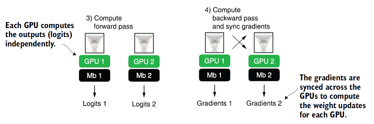
In DDP, the forward and backward passes run independently on each GPU with its corresponding subset of the data. Once the forward and backward passes are done, the gradients of each model replica (on each GPU) are synchronized across all the GPUs. This guarantees that every model replica has the same updated weights. Source: Raschka (2024).

The benefit of using DDP is the speedup it brings to processing the dataset compared with a single GPU. Apart from a small communication overhead between the devices (inherent to DDP), it can theoretically process a training epoch in half the time with two GPUs compared with one. This time saving scales with the number of GPUs, letting us process an epoch eight times faster with eight GPUs, and so on.

Note: DDP does not work properly in interactive Python environments such as Jupyter notebooks, which do not handle multiprocessing the same way a standalone Python script does. The following code must therefore be run as a script, not inside a notebook interface like Jupyter. DDP needs to spawn several processes, and each process must have its own Python interpreter instance.

SELECTING THE AVAILABLE GPUS ON A MULTI-GPU MACHINE

If you want to limit the number of GPUs used for training on a multi-GPU machine, the simplest way is to use the CUDA_VISIBLE_DEVICES environment variable. To illustrate, suppose your machine has several GPUs and you only want to use one of them, for example the GPU with index 0. Instead of python some_script.py, you can run the following command from the terminal:

CUDA_VISIBLE_DEVICES=0 python some_script.py

Or, if your machine has four GPUs and you only want to use the first and the third, you can use:

CUDA_VISIBLE_DEVICES=0,2 python some_script.py

Setting CUDA_VISIBLE_DEVICES this way is a simple and effective way to manage GPU allocation without having to modify your PyTorch scripts.

Duplicated outputs and rank-based control

As the output below shows, the accuracy lines appear twice at the end of a run on a machine with two GPUs:

PyTorch version: 2.2.1+cu117
CUDA available: True
Number of GPUs available: 2
[GPU1] Epoch: 001/003 | Batchsize 002 | Train/Val Loss: 0.60
[GPU0] Epoch: 001/003 | Batchsize 002 | Train/Val Loss: 0.59
[GPU0] Epoch: 002/003 | Batchsize 002 | Train/Val Loss: 0.16
[GPU1] Epoch: 002/003 | Batchsize 002 | Train/Val Loss: 0.17
[GPU0] Epoch: 003/003 | Batchsize 002 | Train/Val Loss: 0.05
[GPU1] Epoch: 003/003 | Batchsize 002 | Train/Val Loss: 0.05
[GPU1] Training accuracy 1.0
[GPU0] Training accuracy 1.0   ← same value, printed twice
[GPU1] Test accuracy 1.0
[GPU0] Test accuracy 1.0       ← same value, printed twice

This behavior is not a bug: it is a direct consequence of how DDP works.

When DDP is used, the Python script is run in full by each process. With two GPUs, two independent processes run at the same time on the machine:

• Process 0 runs the script from start to finish and manages GPU0;
• Process 1 runs the same script from start to finish and manages GPU1.

Each process therefore reaches the line:

print(f"Training accuracy {accuracy}")

and runs it independently. The terminal shows the combined output of both processes, which produces the duplicated lines we see.

We can also see that both processes print the same accuracy. This is not a coincidence: it is the direct consequence of the gradient synchronization DDP performs at every batch:

1. each GPU computes the gradients on its share of the data;
2. DDP averages these gradients across all the processes (AllReduce);
3. each GPU updates its weights with that same average.

Both models therefore receive exactly the same update at every step, end up with identical weights at the end of training, and necessarily produce the same accuracy on the test set.

Printing both results is therefore completely redundant. To fix this, DDP gives each process a rank, that is, a unique ID number (0, 1, 2, …). All we need to do is make the printing conditional on the lead process:

if rank == 0:
    print(f"Test accuracy: {accuracy}")

Process 1 reads this condition, sees that it is not rank 0, and produces no output. Only process 0 prints, and the duplicates disappear.

This is a general rule with DDP: any operation that must happen only once (saving a checkpoint, logging metrics, printing results) must be guarded by an if rank == 0.

Alternatives to DDP for multi-GPU training

DDP is not the only way to train a model on several GPUs with PyTorch. If you prefer a simpler, less verbose approach, companion libraries such as Fabric (open source) achieve the same result with much less boilerplate code.

The author also mentions two advanced techniques covered in the article “Accelerating PyTorch Model Training: Using Mixed-Precision and Fully Sharded Data Parallelism” (available at https://mng.bz/jXle):

• mixed precision: instead of running every computation in float32 (32 bits), some operations are performed in float16 (16 bits). Computations are faster and the GPU memory used by these operations is halved, with a precision loss that is negligible in practice for training.

• Fully Sharded Data Parallelism (FSDP): an extension of DDP in which not only the data but also the model weights themselves are distributed across the GPUs. Each GPU stores only a fraction of the parameters. This makes it possible to train models far too large to fit entirely in the VRAM of a single GPU, which is precisely the case for very large language models.

These two techniques therefore address different problems: mixed precision speeds up and lightens training, while FSDP pushes back the size limit of the models that can be trained.

Summary

• Tensors are PyTorch’s core data structure. .reshape() works in every case, while .view() requires a tensor that is contiguous in memory, which is no longer true after a transposition.
• Autograd builds a computation graph during the forward pass and applies the chain rule to get the gradients, either on demand with grad or for every parameter with .backward().
• A neural network is defined by subclassing torch.nn.Module: the layers in __init__, the flow of data in forward. Models return logits, and the softmax is applied by the loss function.
• Dataset and DataLoader separate reading the examples from assembling them into batches. Workers, shared memory and pin_memory prepare the next batches while the GPU computes.
• The training loop chains the forward pass, the loss, zero_grad(), backward() and step(). model.train() and model.eval() switch the behavior of layers such as dropout.
• Saving a model means saving its state_dict, then loading it back into an instance of the same architecture.
• On a GPU, the model and the data must be on the same device. Beyond one GPU, DDP replicates the model and synchronizes gradients with AllReduce, while model parallelism splits the model itself when it no longer fits on a single GPU.